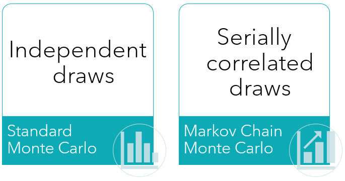
The Metropolis-Hastings algorithm is one of the most popular Markov Chain Monte Carlo (MCMC) algorithms.
Like other MCMC methods, the Metropolis-Hastings algorithm is used to generate serially correlated draws from a sequence of probability distributions. The sequence converges to a given target distribution.
![]()
Table of contents
Before reading this lecture, you should review the basics of Markov chains and MCMC.
In particular, you should keep in mind that an MCMC algorithm generates a
random sequence
![]() having the following properties:
having the following properties:
it is a Markov chain (given
![]() ,
the subsequent observations
,
the subsequent observations
![]() are conditionally independent of the previous observations
are conditionally independent of the previous observations
![]() ,
for any positive integers
,
for any positive integers
![]() and
and
![]() ).
).
two observations
![]() and
and
![]() are in general not
independent,
but they become closer and closer to being independent as
are in general not
independent,
but they become closer and closer to being independent as
![]() increases;
increases;
the sequence converges to the target distribution (the larger
![]() is, the more the distribution of
is, the more the distribution of
![]() is similar to the target distribution).
is similar to the target distribution).
When we run an MCMC algorithm for
![]() periods, we obtain an MCMC sample made up of the
realizations of the
first
periods, we obtain an MCMC sample made up of the
realizations of the
first
![]() terms of the
chain:
terms of the
chain:![]()
Then, we use the empirical distribution of the sample to approximate the target distribution.
Let
![]() be the probability density (or probability mass) function of the distribution
from which we wish to extract a sample of draws. We call
be the probability density (or probability mass) function of the distribution
from which we wish to extract a sample of draws. We call
![]() the target distribution.
the target distribution.
Denote by
![]() a family of conditional distributions of our choice, from which it is easy to
generate draws.
a family of conditional distributions of our choice, from which it is easy to
generate draws.
The vectors
![]() ,
,
![]() and the argument of
and the argument of
![]() all have the same dimension.
all have the same dimension.
The Metropolis-Hastings algorithm starts from any value
![]() belonging to the support of the target distribution. The value
belonging to the support of the target distribution. The value
![]() can be user-defined or extracted from a given distribution.
can be user-defined or extracted from a given distribution.
Then, the subsequent values
![]() are generated recursively.
are generated recursively.
In particular, the value
![]() at time step
at time step
![]() is generated as follows:
is generated as follows:
draw
![]() from the distribution with density
from the distribution with density
![]() ;
;
set![[eq5]](data:image/gif;base64,R0lGODlhAQABAIAAANvf7wAAACH5BAEAAAAALAAAAAABAAEAAAICRAEAOw==)
draw
![]() from a uniform
distribution on
from a uniform
distribution on
![]() ;
;
if
![]() ,
set
,
set
![]() ;
otherwise, set
;
otherwise, set
![]() .
.
Since
![]() is uniform,
is uniform,
![]() that
is, the probability of accepting the proposal
that
is, the probability of accepting the proposal
![]() as the new draw
as the new draw
![]() is equal to
is equal to
![]() .
.
The following terminology is used:
the distribution
![]() is called proposal distribution;
is called proposal distribution;
the draw
![]() is called proposal;
is called proposal;
the probability
![]() is called acceptance probability;
is called acceptance probability;
when
![]() and
and
![]() ,
we say that the proposal is accepted;
,
we say that the proposal is accepted;
when
![]() and
and
![]() ,
we say that the proposal is rejected.
,
we say that the proposal is rejected.
If
![]() for any value of
for any value of
![]() and
and
![]() ,
then we say that the proposal distribution is symmetric.
,
then we say that the proposal distribution is symmetric.
In this special case, the acceptance probability
isand
the algorithm is called Metropolis algorithm.
This simpler version of the algorithm was invented by Nicholas Metropolis.
We do not give a fully rigorous proof of convergence, but we provide the main intuitions.
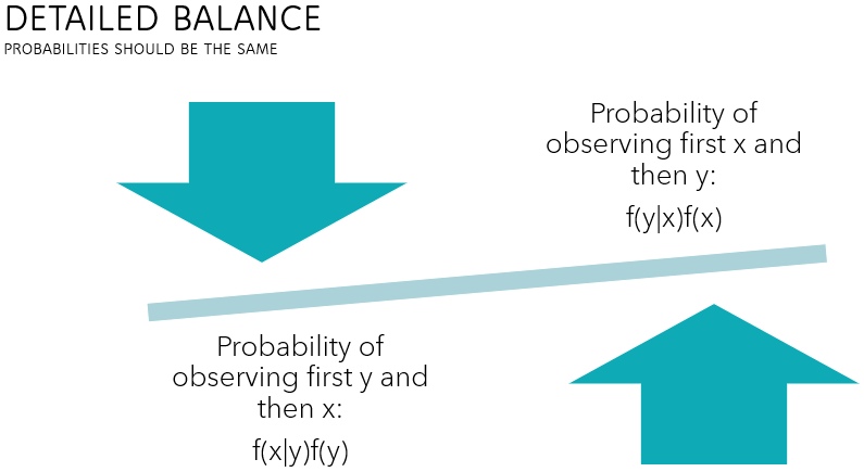
The crucial step is to prove that the so-called detailed balance condition holds (see Markov chains), which implies that the target distribution is the stationary distribution of the Markov chain generated by the Metropolis-Hastings algorithm.
Denote by
![]() the transition kernel of the Markov chain, that is, the probability density of
a transition from
the transition kernel of the Markov chain, that is, the probability density of
a transition from
![]() to
to
![]() .
.
When
![]() ,
then
,
then
![]() and we have
and we have
![[eq11]](/images/Metropolis-Hastings-algorithm__55.png)
Symmetrically, when the transition is from
![]() to
to
![]() and
and
![]() ,
we have
,
we have
![[eq12]](/images/Metropolis-Hastings-algorithm__59.png)
Therefore, when
![]() ,
the target density
,
the target density
![]() and the transition kernel of the chain satisfy the detailed balance
condition
and the transition kernel of the chain satisfy the detailed balance
condition![]()
When
![]() ,
then the detailed balance condition is trivially satisfied because
,
then the detailed balance condition is trivially satisfied because
![]() and
and![]()
By putting together the two cases
(![]() and
and
![]() ),
we find that the detailed balance condition is always satisfied. As a
consequence,
),
we find that the detailed balance condition is always satisfied. As a
consequence,
![]() is the stationary distribution of the chain.
is the stationary distribution of the chain.
When we proved the detailed balance condition, we omitted an important detail: the proposal distribution must be able to generate all the values belonging to the support of the target distribution.
This is intuitive: if the proposal distribution never generates a value
![]() to which the target distribution assigns a positive probability, then
certainly the stationary distribution of the chain cannot be equal to the
target distribution.
to which the target distribution assigns a positive probability, then
certainly the stationary distribution of the chain cannot be equal to the
target distribution.
From a technical viewpoint, if a value
![]() belongs to the support of the target distribution but is never extracted from
the proposal distribution, then
belongs to the support of the target distribution but is never extracted from
the proposal distribution, then
![]() ,
which causes division by zero problems in the proof of the detailed balance
condition and makes it invalid.
,
which causes division by zero problems in the proof of the detailed balance
condition and makes it invalid.
Denote by
![]() the support of the
target density
the support of the
target density
![]() .
.
A simple condition that guarantees that all the values belonging to
![]() can be generated as proposals is that
can be generated as proposals is that
![]() for
any two values
for
any two values
![]() .
.
Not only this condition is sufficient to prove that the target distribution is the stationary distribution of the chain, but it is basically all we need to prove that the chain is ergodic (i.e., we can rely on Law of Large Numbers for dependent sequences) and converges to the stationary distribution.
For a discussion of this condition (and other minor technical conditions that are always satisfied in practice) see Robert and Casella (2013).
As already shown in the introductory lecture on
MCMC
methods, one of the main advantages of the Metropolis-Hastings algorithm
is that we need to know the target distribution
![]() only up to a multiplicative constant.
only up to a multiplicative constant.
This is very important in Bayesian inference, where the posterior distribution is often known up to a multiplicative constant (because the likelihood and the prior are known but the marginal distribution is not).
Suppose
that![]() where
where
![]() is a known function but the constant
is a known function but the constant
![]() is not.
is not.
Then, the acceptance probability
is![[eq19]](/images/Metropolis-Hastings-algorithm__81.png)
So, we do not need to know the constant
![]() to compute the acceptance probability, and the latter is the only quantity in
the algorithm that depends on the target distribution
to compute the acceptance probability, and the latter is the only quantity in
the algorithm that depends on the target distribution
![]() .
.
Therefore, we can use the Metropolis-Hastings algorithm to generate draws from a distribution even if we do not fully know the probability density (or mass) of that distribution!
If the proposal
![]() is independent of the previous state
is independent of the previous state
![]() ,
that
is,
,
that
is,![]() then
the algorithm is called Independent Metropolis-Hastings or
Independence chain Metropolis-Hastings.
then
the algorithm is called Independent Metropolis-Hastings or
Independence chain Metropolis-Hastings.
For example, a common choice is to extract proposals
![]() from a
multivariate
normal distribution (each draw is independent from the previous ones).
from a
multivariate
normal distribution (each draw is independent from the previous ones).
When
![]() is drawn independently, the acceptance probability is
is drawn independently, the acceptance probability is
It is easy to see that
![]() when
when
![]() for any
for any
![]() .
.
In other words, if the proposal distribution is equal to the target
distribution, the acceptance probability is
![]() and the proposal is always accepted. Furthermore, since the
proposals are independent, we obtain a sample of independent draws from the
target distribution.
and the proposal is always accepted. Furthermore, since the
proposals are independent, we obtain a sample of independent draws from the
target distribution.
On the contrary, the more the proposal distribution differs from the target distribution, the lower the acceptance probabilities are, and the more often the proposals are rejected.
The consequence is that the chain remains stuck at particular points for long periods of time, giving rise to a highly serially correlated MCMC sample.
As discussed in the lecture on MCMC diagnostics, chains that produce highly correlated samples can be problematic because they need to be run for very long periods of time, which can be prohibitively costly.
Therefore, the proposal distribution should be as similar as possible to the target distribution, so as to get high acceptance probabilities and samples with low serial correlation.
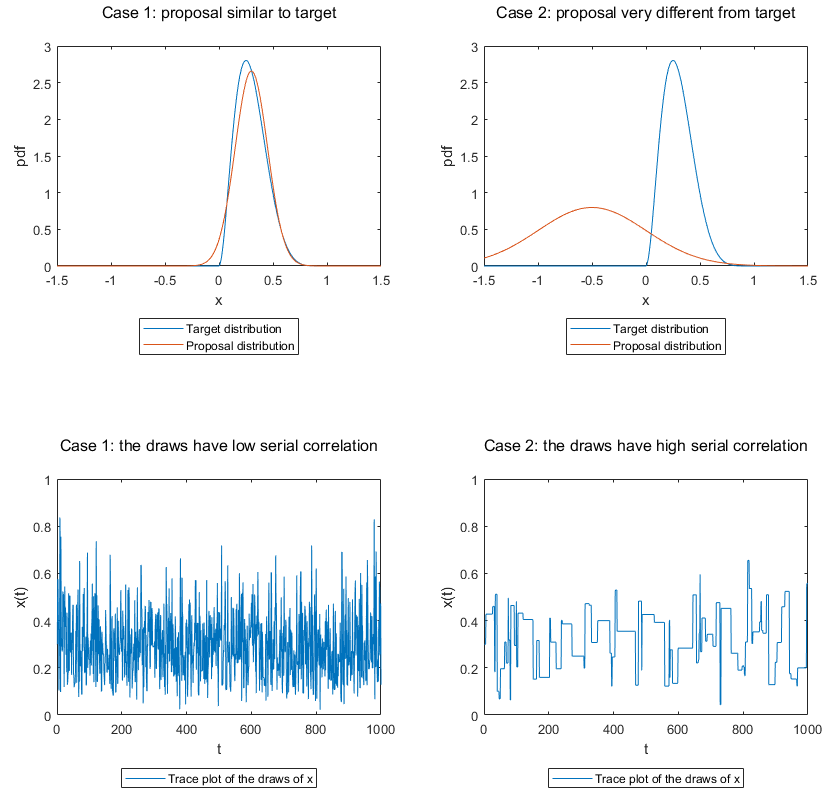
In the following plot, we show two examples:
on the left, the proposal is close to the target (upper panel); as a consequence, the samples are only mildly correlated (lower panel);
on the right, the proposal is very different from the target (upper panel); as a consequence, the samples are highly correlated (lower panel).
Unfortunately, there is no simple and universal method to select good proposal distributions. In fact, this is a topic that is still actively researched by statisticians.
However, a generally valid strategy is to:
start with a simple proposal distribution (e.g., a multivariate normal);
generate a first MCMC sample (which might be too correlated) and use it to infer characteristics of the target distribution (e.g., its mean and covariance matrix);
use the things learned from the first sample to improve the proposal distribution (e.g., by tuning the mean and covariance of the multivariate normal used as proposal).
If the proposals are formed
as![]() where
where
![]() is a sequence of independent draws from a known probability distribution
(e.g., multivariate normal), then the algorithm is called Random walk
Metropolis-Hastings.
is a sequence of independent draws from a known probability distribution
(e.g., multivariate normal), then the algorithm is called Random walk
Metropolis-Hastings.
We have
that![]() and
and![]()
Therefore, the acceptance probability
is![[eq27]](/images/Metropolis-Hastings-algorithm__98.png)
To understand the properties of this algorithm, let us consider the special
(but very common in practice) case in which the distribution of the random
walk increment
![]() is symmetric.
is symmetric.
In this case,
![]() ,
and the acceptance probability
is
,
and the acceptance probability
is
Suppose also that the target density has the following two characteristics (which are very common in practice too):
points that are close to each other have similar densities;
there is a high probability region (e.g., around the mode of the distribution); the points that are far from this region have a much lower density than the points that belong to it.
Now, consider two extreme cases:
if the random walk increments
![]() are on average very small (their
variance is small), then
the
ratioand
the acceptance probability
are on average very small (their
variance is small), then
the
ratioand
the acceptance probability
![]() are always close to
are always close to
![]() because, by assumption, points that are close to each other have similar
densities; the proposals are almost always accepted, but they are very close
to each other; the resulting MCMC sample is highly serially correlated;
because, by assumption, points that are close to each other have similar
densities; the proposals are almost always accepted, but they are very close
to each other; the resulting MCMC sample is highly serially correlated;
if the random walk increments
![]() are on average very large (their variance is large), then the
ratiois
often close to zero when
are on average very large (their variance is large), then the
ratiois
often close to zero when
![]() lies in the high probability region because the proposals tend to be far from
this region and to have low density; the proposals are often rejected and the
chain remains stuck at high-density points for long periods of time; we obtain
a highly serially correlated MCMC sample.
lies in the high probability region because the proposals tend to be far from
this region and to have low density; the proposals are often rejected and the
chain remains stuck at high-density points for long periods of time; we obtain
a highly serially correlated MCMC sample.
The bottom line is: we get a highly correlated sample both if the variance of the increments is too large and if it is too small.
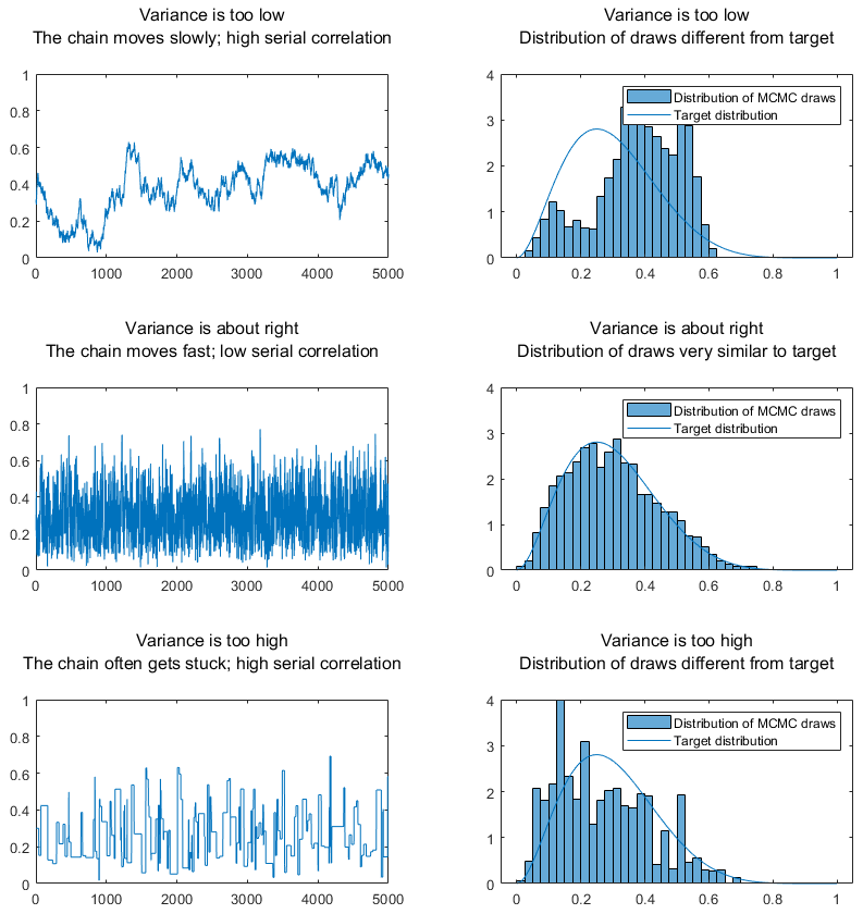
To avoid these two extreme cases, it is very important to accurately tune the variance of the random walk increments.
We can do this, for example, with a trial-and-error process:
we start with a guess of a good value for the variance, and we generate a first MCMC sample;
then, we look at the trace plots of the sample (see MCMC diagnostics); if we see points where the chain gets stuck (flat lines in trace plot) we decrease the variance, while if we see that the trace plot moves very slowly, we increase the variance;
finally, we re-run the chain.
An alternative and very effective method is to automatically tune the variance while running the chain.
Methods to do so are called adaptive Metropolis-Hastings methods. We do not discuss them here, but you can read this nice introduction if you are interested in the topic.
Robert, C. P. and G. Casella (2013) Monte Carlo Statistical Methods, Springer Verlag.
Please cite as:
Taboga, Marco (2021). "Metropolis-Hastings algorithm", Lectures on probability theory and mathematical statistics. Kindle Direct Publishing. Online appendix. https://www.statlect.com/fundamentals-of-statistics/Metropolis-Hastings-algorithm.
Most of the learning materials found on this website are now available in a traditional textbook format.