Markov Chain Monte Carlo (MCMC) diagnostics are tools that can be used to check whether the quality of a sample generated with an MCMC algorithm is sufficient to provide an accurate approximation of the target distribution.
In particular, MCMC diagnostics are used to check:
whether a large portion of the MCMC sample has been drawn from distributions that are significantly different from the target distribution;
whether the size of the generated sample is too small.
![]()
Table of contents
Throughout this lecture we are going to assume that you are familiar with the basics of the Markov Chain Monte Carlo method.
Here are some important facts that you need to keep in mind.
An MCMC algorithm produces a sequence
![]() of random variables (or vectors). The sequence has the following properties:
of random variables (or vectors). The sequence has the following properties:
it is a Markov chain;
the larger
![]() is, the more the distribution of
is, the more the distribution of
![]() is similar to the target distribution (in technical terms, we say that the
chain converges to its stationary distribution, which is by construction equal
to the target distribution);
is similar to the target distribution (in technical terms, we say that the
chain converges to its stationary distribution, which is by construction equal
to the target distribution);
in general, two terms of the chain
![]() and
and
![]() are not
independent.
However, the further apart two terms are in the chain, the closer they are to
being independent from each other. In other words,
are not
independent.
However, the further apart two terms are in the chain, the closer they are to
being independent from each other. In other words,
![]() and
and
![]() become almost independent as
become almost independent as
![]() gets large.
gets large.
When we run an MCMC algorithm for
![]() periods, we get an MCMC sample made up of the first
periods, we get an MCMC sample made up of the first
![]() realizations of the
chain:
realizations of the
chain:![]() and
then we use the empirical
distribution of the sample to approximate the target distribution.
and
then we use the empirical
distribution of the sample to approximate the target distribution.
What kind of problems do MCMC diagnostics try to spot? Basically, there are two main problems that we may encounter.
In general, the distribution of the starting value
![]() is different from the target distribution. As a consequence, also the
distributions of
is different from the target distribution. As a consequence, also the
distributions of
![]() are different from the target distribution, although the differences become
smaller and smaller as
are different from the target distribution, although the differences become
smaller and smaller as
![]() increases because, by construction, the distribution of
increases because, by construction, the distribution of
![]() converges to the target distribution as
converges to the target distribution as
![]() tends to infinity.
tends to infinity.
It can happen that the chain is slow to converge, that is, after many
iterations, the distributions of the draws are still very different from the
target distribution. Typically, this happens when the initial value
![]() lies in a region to which the target distribution assigns a very small
probability.
lies in a region to which the target distribution assigns a very small
probability.
When the chain converges slowly, a large portion of our MCMC sample might be made up of observations drawn from distributions that are significantly different from the target distribution.
If we are able to spot this kind of problem, we can try to fix it by:
discarding a large chunk of initial observations (the so-called burn-in sample);
increasing the number of iterations (i.e., the sample size).
Both of these fixes have the effect of increasing the proportion of draws extracted from distributions that are (more) similar to the target distribution.
Remember that, in general, two terms of the chain
![]() and
and
![]() are not independent. However, they become almost independent as
are not independent. However, they become almost independent as
![]() gets large.
gets large.
Suppose that we are able to find the smallest number
![]() such that, for any
such that, for any
![]() ,
,
![]() and
and
![]() can be considered independent for all practical purposes (their degree of
dependence is negligible). For the sake of simplicity, also assume that the
sample size
can be considered independent for all practical purposes (their degree of
dependence is negligible). For the sake of simplicity, also assume that the
sample size
![]() is a multiple of
is a multiple of
![]() .
Then, we can form a
sub-sample
.
Then, we can form a
sub-sample![]() of
realizations of mutually independent variables. The dimension of this
sub-sample, which we call effective sample size, is
of
realizations of mutually independent variables. The dimension of this
sub-sample, which we call effective sample size, is
![]() .
.
Roughly speaking, the MCMC sample is equivalent to a sample
of independent observations having size
![]() .
The slower the decay of the dependence between the terms of the Markov chain
is, the larger
.
The slower the decay of the dependence between the terms of the Markov chain
is, the larger
![]() ,
and the smaller the effective sample size is.
,
and the smaller the effective sample size is.
When the dependence decays very slowly
(![]() is very large), it easily happens that the effective sample size
(
is very large), it easily happens that the effective sample size
(![]() )
of the MCMC sample is too small, in the sense that the limited size of the
sample makes its empirical distribution a very noisy/imprecise approximation
of the target distribution.
)
of the MCMC sample is too small, in the sense that the limited size of the
sample makes its empirical distribution a very noisy/imprecise approximation
of the target distribution.
If we are able to spot this kind of problem, we can try to fix it by:
tweaking the MCMC algorithm so as to decrease the dependence (decrease
![]() );
);
increasing the number of iterations (i.e., the sample size
![]() ).
).
Both of these fixes have the effect of increasing the effective sample size.
Note: the definition of effective sample size given here is not rigorous and is different from the definition usually found in MCMC textbooks and papers. Its only purpose is to clearly illustrate the problems that can be generated by slowly decaying dependence.
Most MCMC diagnostics test for the absence of Problems 1 and 2 described above.
In particular, absent problems 1 and 2, the following hypotheses hold:
the majority of the observations in the MCMC sample have been drawn from distributions that are very similar to the target distribution;
the effective size of the sample is not too small.
If these two hypotheses hold, then the implication is that:
the empirical distribution of any large chunk of the sample is a good approximation of the target distribution.
By large chunk we mean a sub-sample of adjacent draws representing a significant portion of the overall sample (see Example 1 below).
Many diagnostics are used to test the implication above (call it nice large chunks). If a diagnostic tells us that large chunks are not nice, then our sample is afflicted by either Problem 1 or 2 and its quality is not sufficient.
The simplest way to diagnose problems in an MCMC sample is to split the sample into two or more chunks and check whether we get the same results on all the chunks.
Example
Suppose our MCMC sample is made up of
![]() draws (with
draws (with
![]() even):
even):![]() where
a generic draw
where
a generic draw
![]() is a
is a
![]() random vector. Then, we can divide the sample into two
chunks
random vector. Then, we can divide the sample into two
chunks![[eq6]](/images/Markov-Chain-Monte-Carlo-diagnostics__40.png) and
compute their sample
means
and
compute their sample
means![[eq7]](/images/Markov-Chain-Monte-Carlo-diagnostics__41.png) If
the two sample means are significantly different (we can run a formal
statistical test to check the difference), then this is a symptom that the
quality of our MCMC sample is not sufficient.
If
the two sample means are significantly different (we can run a formal
statistical test to check the difference), then this is a symptom that the
quality of our MCMC sample is not sufficient.
In the previous example, we have compared the sample means of the two sub-samples, but the comparison could be conducted also on other sample moments, for instance, on the sample variances.
The rationale behind this simple diagnostic is very simple. If we find that two chunks of the sample have significantly different empirical distributions, then it must be that at least one of the two is not a good approximation of the target distribution. This contradicts the nice large chunks principle. Therefore, the quality of our sample is not sufficient.
Another simple way to diagnose problems is to run the MCMC algorithm more than
once with different (possibly, very different) starting points
![]() ,
so as to obtain multiple MCMC samples. Then, we check whether we get the same
results on all the samples (possibly, after discarding burn-ins). We can
conduct the checks by testing whether the sample means or other sample moments
are significantly different across the different MCMC samples, similarly to
what we did in the previous section (Sample splits).
,
so as to obtain multiple MCMC samples. Then, we check whether we get the same
results on all the samples (possibly, after discarding burn-ins). We can
conduct the checks by testing whether the sample means or other sample moments
are significantly different across the different MCMC samples, similarly to
what we did in the previous section (Sample splits).
Trace plots may help us to understand what kind of problem (if any) affects our MCMC sample.
Suppose our MCMC sample is made up of
![]() draws
draws![]() where
a generic draw
where
a generic draw
![]() is a
is a
![]() random vector.
random vector.
A trace plot is a line chart that has:
time
(![]() )
on the x-axis;
)
on the x-axis;
the values taken by one of the coordinates of the draws (e.g.,
![]() if the
if the
![]() -th
coordinate is plotted) on the y-axis.
-th
coordinate is plotted) on the y-axis.
The next figure contains three trace plots that illustrate typical situations we may encounter.
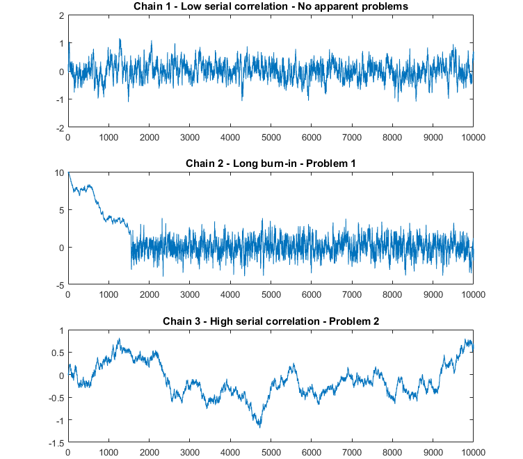
In the first trace plot (Chain 1), there are no apparent anomalies. There seems to be a mild serial correlation between successive draws and the chain seems to explore the sample space many times.
In the second plot (Chain 2), the first part of the sample (until around
![]() )
looks very different from the remaining part. Most likely, the initial
distribution and the distributions of the subsequent terms of the chain were
very different from the target distribution, but then the chain slowly
converged to the target distribution (around
)
looks very different from the remaining part. Most likely, the initial
distribution and the distributions of the subsequent terms of the chain were
very different from the target distribution, but then the chain slowly
converged to the target distribution (around
![]() ).
We have Problem 1: a large chunk of the sample is drawn from distributions
that are significantly different from the target distribution.
).
We have Problem 1: a large chunk of the sample is drawn from distributions
that are significantly different from the target distribution.
In the third plot (Chain 3), there is a lot of serial correlation between successive draws. The chain is very slow in exploring the sample space. The sample space has been explored only few times. In other words, there seems to be few independent observations in our sample. Quite likely, we have Problem 2: the effective size of our sample is too small.
The next two trace plots show how Problem 1 and 2 can be solved.
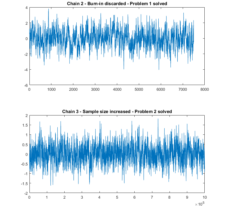
In the first plot, the same sample from Chain 2 is used, but the burn-in (the
first
![]() observations) is discarded.
observations) is discarded.
In the second plot, a new sample from Chain 3 is generated, but the sample
size is increased dramatically (from
![]() to
to
![]() draws) so as to increase the effective sample size and let the chain explore
the sample space many times.
draws) so as to increase the effective sample size and let the chain explore
the sample space many times.
In both cases, problems seem to have been solved: the trace plots of the MCMC samples do not show any apparent anomaly.
We note that, although trace plots are pretty simple and informal diagnostic tools, they seem to be the most frequently used: if you are trying to publish an MCMC study in a scientific journal, it is very likely that you will be asked to include your trace plots in the study!
By inspecting trace plots, we can get a sense of the degree of serial correlation of the draws. To measure serial correlation precisely, we can use so-called ACF (autocorrelation function) plots, also called correlograms. From these plots you can see how the sample autocorrelation between the terms of the chain decreases as a function of their lag (see the lecture on autocorrelation for more details).
The next figure contains the sample ACF plots of the three MCMC samples whose trace plots have been discussed in the previous section.
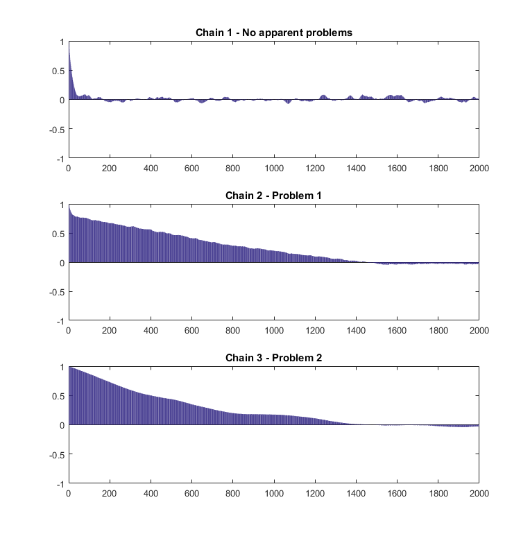
The ACF plot of Chain 1 shows that autocorrelation is large at short lags, but then goes to zero pretty quickly (remember that the trace plot did not provide evidence of any problems).
The plots of Chains 2 and 3 show that not only autocorrelation is large at short lags, but it also dies out very slowly. Interestingly the sample ACFs of Chains 2 and 3 are quite similar, even if the trace plots provide evidence that the two chains are affected by different problems (Problems 1 and 2 respectively). According to our experience, this is something that happens quite frequently. Although ACF plots help us to assess the presence of problems and allow us to better quantify autocorrelation, it is difficult to tell from ACFs what the problem is. Therefore, it is advisable to use trace plots and ACF plots together.
We should note that MCMC experts generally agree on the following facts:
no single diagnostic is perfect;
we can never be 100% sure that the quality of an MCMC sample is adequate (diagnostics can help us to spot a problem, but they cannot guarantee the absence of problems).
For these reasons, the best thing we can do is to analyze our MCMC samples as accurately as possible and to employ many different diagnostics to assess their quality.
Having said that performing many diagnostics is always a good idea, we feel like giving another piece of advice: always run your chains for as long as you can, run many chains with different starting points, and do not spare computational resources. This is the best way to avoid problems.
Please cite as:
Taboga, Marco (2021). "Markov Chain Monte Carlo (MCMC) diagnostics", Lectures on probability theory and mathematical statistics. Kindle Direct Publishing. Online appendix. https://www.statlect.com/fundamentals-of-statistics/Markov-Chain-Monte-Carlo-diagnostics.
Most of the learning materials found on this website are now available in a traditional textbook format.