A statistical model is a set of assumptions about the probability distribution that generated some observed data.
![]()
Table of contents
We provide here some examples of statistical models.
Example
Suppose that we randomly draw
![]() individuals from a certain population and measure their height. The
measurements can be regarded as
realizations of
individuals from a certain population and measure their height. The
measurements can be regarded as
realizations of
![]() random variables
random variables
![]() .
In principle, these random variables could have any probability distribution.
If we assume that they have a
normal
distribution, as it is often done for height measurements, then we are
formulating a statistical model: we are placing a restriction on the set of
probability distributions that could have generated the data.
.
In principle, these random variables could have any probability distribution.
If we assume that they have a
normal
distribution, as it is often done for height measurements, then we are
formulating a statistical model: we are placing a restriction on the set of
probability distributions that could have generated the data.
Example
In the previous example, the random variables
![]() could have some form of dependence. If we assume that they are
statistically
independent, then we are placing a further restriction on their joint
distribution, that is, we are adding an assumption to our statistical model.
could have some form of dependence. If we assume that they are
statistically
independent, then we are placing a further restriction on their joint
distribution, that is, we are adding an assumption to our statistical model.
Example
Suppose that for the same
![]() individuals we also collect weight measurements
individuals we also collect weight measurements
![]() ,
and we assume that there is a linear relation between weight and height,
described by a
regression
equation
,
and we assume that there is a linear relation between weight and height,
described by a
regression
equation![]() where
where
![]() and
and
![]() are regression coefficients and
are regression coefficients and
![]() is an error term. This is a statistical model because we have placed a
restriction on the set of joint distributions that could have generated the
couples
is an error term. This is a statistical model because we have placed a
restriction on the set of joint distributions that could have generated the
couples
![]() :
we have ruled out all the joint distributions in which the two variables have
a relation that cannot be described by the regression equation.
:
we have ruled out all the joint distributions in which the two variables have
a relation that cannot be described by the regression equation.
Example
If we assume that all the errors
![]() in the previous regression equation have the same
variance (i.e., the
errors are not heteroskedastic),
then we are placing a further restriction on the set of data-generating
distributions. Thus, we have yet another statistical model.
in the previous regression equation have the same
variance (i.e., the
errors are not heteroskedastic),
then we are placing a further restriction on the set of data-generating
distributions. Thus, we have yet another statistical model.
![[eq6]](/images/statistical-model__25.png)
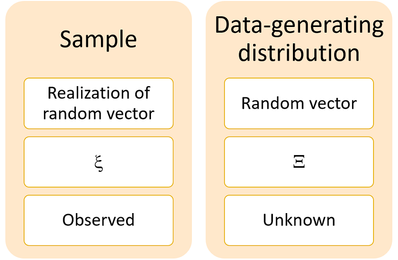
As shown in the previous examples, a model is a set of probability distributions that might have generated the data sample.
The sample, denoted by
![]() ,
is a vector of data. It can be thought of as the
realization of a
random vector
,
is a vector of data. It can be thought of as the
realization of a
random vector
![]() .
.
In principle,
![]() could have any joint
probability distribution.
could have any joint
probability distribution.
If we assume that the distribution of
![]() belongs to a certain set of distributions
belongs to a certain set of distributions
![]() ,
then
,
then
![]() is called a statistical model (see, e.g., McCullagh
2002).
is called a statistical model (see, e.g., McCullagh
2002).
When the statistical model
![]() is put into correspondence with a set
is put into correspondence with a set
![]() of real vectors, then we have a parametric model.
of real vectors, then we have a parametric model.
The set
![]() is called parameter space and any one
of its members
is called parameter space and any one
of its members
![]() is called a parameter.
is called a parameter.
Example
Assume, as we did in the first example above, that the height measurements
![]() come from a normal distribution. Then,
come from a normal distribution. Then,
![]() is the set of all normal distributions. But a normal distribution is
completely characterized by its mean
is the set of all normal distributions. But a normal distribution is
completely characterized by its mean
![]() and its variance
and its variance
![]() .
As a consequence, each member of
.
As a consequence, each member of
![]() is put in correspondence with a vector of parameters
is put in correspondence with a vector of parameters
![]() .
The mean
.
The mean
![]() can take any real value and the variance
can take any real value and the variance
![]() needs to be positive. Therefore, the parameter space is
needs to be positive. Therefore, the parameter space is
![]() .
.
When a correspondence between
![]() and a parameter space is not specified, then we have a nonparametric model.
and a parameter space is not specified, then we have a nonparametric model.
In this case, we use techniques that allow us to directly analyze
![]() ,
for example:
,
for example:
multivariate kernel density estimation (the distribution of the data is recovered through histogram-like estimators);
kernel regression (the joint distribution estimated with kernel density methods is used to derive the distribution of some variables conditional on others).
These models, used in nonparametric statistics, make minimal assumptions about the data-generating distribution. They allow the data to "speak for themselves" (e.g., Hazelton 2015).
What do we do after formulating a parametric statistical model?
The typical things we do are:
parameter
estimation: we produce a guess of the parameter
![]() associated to the true distribution (the one that generated the data); the
guess is produced using so-called
estimation
methods, such as:
associated to the true distribution (the one that generated the data); the
guess is produced using so-called
estimation
methods, such as:
set estimation: we
search for a small subset of
![]() that contains the true parameter
that contains the true parameter
![]() with high probability;
with high probability;
hypothesis testing: we place further restrictions on the set of possible data-generating distributions; then, we test whether the restrictions are supported by the data;
Bayesian updating: we first assign a prior distribution to the parameters; then we use the sample data to update the distribution.
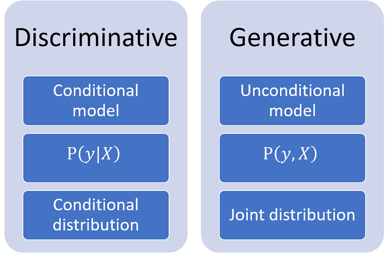
In conditional models (also called discriminative models), the sample is partitioned into input and output data, as in the regression example above. The statistical model is obtained by placing some restrictions on the conditional probability distribution of the outputs given the inputs.
This is in contrast to unconditional models (also called generative models), used to analyze the joint distribution of inputs and outputs.
There are two classes of conditional models:
regression models, in which the output variable is continuous; for example:
the linear regression model, which postulates the existence of a linear relation between the outputs (dependent variables) and the inputs (explanatory variables);
non-linear regression, in which the input-output mapping can be non-linear.
classification models, in which the output variable is discrete (or categorical); for example:
the logistic classification model (or logit model), used to model the influence of some explanatory variables on a binary outcome;
the multinomial logit, in which the response variable can take more than two discrete values.
Understanding the distinction between regression and classification is essential for a correct choice of a statistical model.
Conditional statistical models can be used to make predictions of unseen outputs given observed inputs.
There are models that also allow us to make such predictions, but without specifying a set of conditional probability distributions (not even implicitly). Strictly speaking, they are not statistical models. They can be broadly classified as predictive models.
Predictive models can be seen as algorithms that try to accurately reproduce a mapping between inputs and outputs (see, e.g., Breiman 2001).
Several models used in the machine learning field belong to the class of predictive models. For example:
A fundamental characteristic of a parametric statistical model is the
dimension of its parameter space
![]() ,
which is equal to the number of entries of the parameter vectors
,
which is equal to the number of entries of the parameter vectors
![]() .
.
Example The dimension of a linear regression model is equal to the number of regression coefficients, which in turn is equal to the number of input variables.
Models that have a large dimension are often difficult to estimate, as the estimators of the parameter vector tend to have high variance.
Moreover, large models are prone to over-fitting: they tend to accurately fit the sample data, and to poorly predict out-of-sample data.
For these reasons, we often try to specify parsimonious statistical models, that is, simple models with few parameters. Despite its simplicity, a parsimonious model should be able to reproduce all the main characteristics of the data in a satisfactory manner.
Techniques used to obtain parsimonious specifications and fight over-fitting include:
parameter regularization methods, used to reduce the variance of parameter estimators; for example:
variable selection methods, used to discard input variables that are unlikely to be relevant; for example:
A statistician might formulate more than one statistical model.
The choice among alternative models can be performed using:
model selection criteria, that rank the models based on their estimated distance from the data-generating distribution;
cross validation, in which validation samples not used for estimation are employed to compare the predictive accuracy of the models;
hierarchical Bayesian methods, that allow us to compute the posterior odds of different models.
We have said above that a statistical model
![]() is a set of probability distributions.
is a set of probability distributions.
A model is said to be correctly specified if
![]() includes the true data-generating distribution. Otherwise, it is said to be
misspecified.
includes the true data-generating distribution. Otherwise, it is said to be
misspecified.
There are numerous diagnostics, statistical tests and metrics used to detect misspecification.
Some examples are:
the Cramér-von Mises test, which detects significant differences between an hypothesized distribution and the true distribution of the data;
the PRESS statistic, used to assess the ability of a model to predict out-of-sample data;
the Ramsey RESET test, which detects important nonlinearities ignored by the model;
the Hosmer-Lemeshow test, which evaluates the correct calibration of classification models;
the F test, which can be used to test whether some input variables have been unduly excluded from a regression model;
residual plots, diagnostic tools used to check for violations of assumptions in a linear regression.
More details about the mathematics of statistical modelling can be found in the lecture on statistical inference.
Breiman, L., 2001. Statistical modeling: The two cultures (with comments and a rejoinder by the author). Statistical science, 16(3), pp.199-231.
Hazelton, M. L., 2015. Nonparametric regression. International Encyclopedia of the Social & Behavioral Sciences (Second Edition), pp. 867-877
McCullagh, P., 2002. What is a statistical model? The Annals of Statistics, 30(5), pp.1225-1310.
Previous entry: Stationary sequence
Next entry: Support of a random variable
Please cite as:
Taboga, Marco (2021). "Statistical model", Lectures on probability theory and mathematical statistics. Kindle Direct Publishing. Online appendix. https://www.statlect.com/glossary/statistical-model.
Most of the learning materials found on this website are now available in a traditional textbook format.