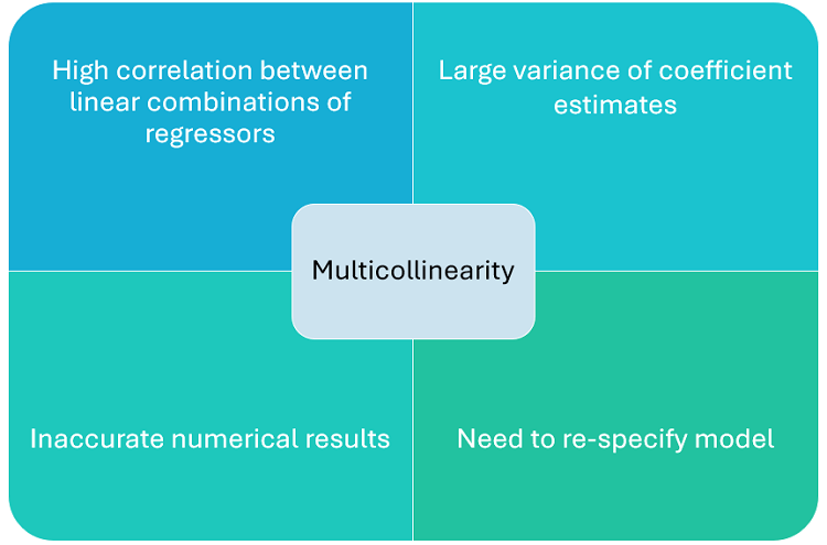
Multicollinearity is a problem that affects linear regression models in which one or more of the regressors are highly correlated with linear combinations of other regressors.
When this happens, the OLS estimator of the regression coefficients tends to be very imprecise, that is, it has high variance, even if the sample size is large.
![]()
Before speaking about multicollinearity, let us introduce the notation we are going to use:
the
![]() vector of observations of
the dependent variable is denoted by
vector of observations of
the dependent variable is denoted by
![]() ;
;
the
![]() design matrix, that is, the matrix of regressors, is denoted by
design matrix, that is, the matrix of regressors, is denoted by
![]() ;
;
the
![]() vector of regression coefficients is denoted by
vector of regression coefficients is denoted by
![]() ;
;
the
![]() vector of errors is denoted by
vector of errors is denoted by
![]() .
.
The regression equation in matrix form
is![]()
The OLS estimator
![]() is the solution to the minimization
problem
is the solution to the minimization
problem![[eq2]](/images/multicollinearity__11.png)
When
![]() has full rank, the solution
is
has full rank, the solution
is![]()
Under certain conditions, the
covariance
matrix of the OLS estimator
is![]() where
where
![]() is the variance of
is the variance of
![]() for
for
![]() .
.
In particular, this formula for the covariance matrix holds exactly in the normal linear regression model and asymptotically under the conditions stated in the lecture on the properties of the OLS estimator.
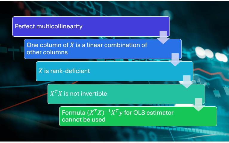
The most extreme case is that of perfect multicollinearity, in which at least one regressor can be expressed as a linear combination of other regressors.
In this case, one of the columns of
![]() can be written as a linear
combination of the other columns.
can be written as a linear
combination of the other columns.
As a consequence,
![]() is not full-rank and, by some
elementary results on
matrix products and
ranks, the rank of the product
is not full-rank and, by some
elementary results on
matrix products and
ranks, the rank of the product
![]() is less than
is less than
![]() ,
so that
,
so that
![]() is not invertible. Thus, the
formula for the OLS estimator cannot even be computed.
is not invertible. Thus, the
formula for the OLS estimator cannot even be computed.
Roughly speaking, trying to invert a rank deficient matrix is like trying to compute the reciprocal of zero.
In the case of perfect multicollinearity, we try to compute the variances in
equation (1), and we incur into a division-by-zero problem: we divide
![]() by zero and, as a consequence, the variances of the regression coefficients
(the diagonal elements of
by zero and, as a consequence, the variances of the regression coefficients
(the diagonal elements of
![]() )
go to infinity.
)
go to infinity.
When one of the regressors is highly correlated with, but not equal to a linear combination of other regressors, then we say that the regression suffers from multicollinearity, although the multicollinearity is not perfect.
In such a case the design matrix is full-rank, but it is not very far from being rank-deficient.
Continuing with the division-by-zero analogy above, when multicollinearity is
not perfect, we are dividing
![]() in equation (1) by a number that is very small, so that the variances of the
regression coefficients are very large.
in equation (1) by a number that is very small, so that the variances of the
regression coefficients are very large.
Ho do we measure the degree of multicollinearity? How do we make the definition of non-perfect multicollinearity above more precise?
The degree of multicollinearity is usually measured separately for each
regressor
![]() (
(![]() ),
by comparing two quantities:
),
by comparing two quantities:
the variance that
![]() (the OLS estimate of the coefficient of
(the OLS estimate of the coefficient of
![]() in the regression being estimated) would have if
in the regression being estimated) would have if
![]() was uncorrelated with all the other regressors;
was uncorrelated with all the other regressors;
the actual variance of
![]() .
.
The ratio between these two quantities (actual/hypothetical variance) is called variance inflation factor (VIF).
The VIF measures by how much the linear correlation of a given regressor with the other regressors increases the variance of its coefficient estimate with respect to the baseline case of no correlation.
It can be proved that the variance inflation factor for the coefficient
![]() is
is![[eq9]](/images/multicollinearity__33.png) where
where
![]() is the
R
squared of a regression in which
is the
R
squared of a regression in which
![]() is the dependent variable and
is the dependent variable and
![]() (
(![]() )
are the dependent variables.
)
are the dependent variables.
If the regressor being examined is highly correlated with a linear combination
of the other regressors, then
![]() is close to 1 and the variance inflation factor is large.
is close to 1 and the variance inflation factor is large.
In the limit, when
![]() tends to 1, that is, in the case of perfect multicollinearity examined above,
tends to 1, that is, in the case of perfect multicollinearity examined above,
![]() tends to infinity.
tends to infinity.
Although no rule of thumb is perfect (see O'Brien
2007), values of the VIF above 10 (i.e.,
![]() )
are often considered an indication that it might be worthwhile to adopt a
remedy to reduce multicollinearity (see below).
)
are often considered an indication that it might be worthwhile to adopt a
remedy to reduce multicollinearity (see below).
For more details, see the lecture on the VIF.

There is an important and often overlooked issue about multicollinearity: when
![]() is close to being singular, the result of calculating the
inverse
is close to being singular, the result of calculating the
inverse![]() on
a computer can be severely biased by numerical error.
on
a computer can be severely biased by numerical error.
This is very important: even if we are comfortable with a high VIF and we are willing to tolerate the fact that the linear correlation among the regressors is inflating the variance of our OLS estimates, we should nonetheless check that multicollinearity is not a potential source of large numerical errors.
In the next section we show how to do this check.
The condition number is the statistic most commonly used to check whether the
inversion of
![]() may cause numerical problems.
may cause numerical problems.
Here we provide an intuitive introduction to the concept of condition number, but see Brandimarte (2007) for a formal but easy-to-understand introduction.
Consider the OLS estimate
![]()
Since computers perform finite-precision arithmetic, they introduce round-off
errors in the computation of products and additions such as those in the
matrix product
![]() .
.
In turn, these round-off errors are amplified (or dampened)
when we multiply
![]() by the inverse
by the inverse
![]() .
By how much are the errors amplified?
.
By how much are the errors amplified?
The condition number of
![]() tells us by how much they are amplified in the worst possible case.
tells us by how much they are amplified in the worst possible case.
For example, if the condition number equals 100, then there are cases in which
the round-off error in the computation of
![]() is amplified 100-fold when multiplying it by
is amplified 100-fold when multiplying it by
![]() .
.
While there are no precise rules, some authors (e.g.,
Greene 2000) suggest that multicollinearity is
likely to cause numerical problems if the condition number of
![]() is greater than 20.
is greater than 20.
Most statistical packages have built-in functions to compute the condition number of a matrix. For details on the computation of the condition number, see Brandimarte (2007).
What do we do to deal with multicollinearity?
In the case of perfect multicollinearity, at least one regressor is a linear combination of the other regressors. In other words, it is redundant and it does not add any information.
Then, the remedy is to simply drop it from the regression.
When multicollinearity is not perfect, the following remedies may be considered:
increase the sample size; by doing so,
the variance of the OLS estimates tends to decrease, even if it is inflated by
high correlation among regressors; furthermore, a larger sample size decreases
over-fitting and tends to reduce
![]() (see
this
lecture for a discussion of the impact of over-fitting on the R squared of
a linear regression);
(see
this
lecture for a discussion of the impact of over-fitting on the R squared of
a linear regression);
drop one or more regressors that have a high VIF if they are not deemed to be essential;
replace highly correlated regressors with a linear combination of them;
use regularization methods such as ridge and lasso;
use Bayesian regression; if multicollinearity prevents a regression coefficient from being estimated precisely, then the prior on that coefficient will help to reduce its posterior variance.
Brandimarte, P. (2006) Numerical Methods in Finance and Economics: A MATLAB-Based Introduction, 2nd Edition, Wiley Interscience.
Greene, W.H. (2002) Econometric analysis, 5th edition. Prentice Hall.
O'Brien, R. (2007) A Caution Regarding Rules of Thumb for Variance Inflation Factors, Quality & Quantity, 41, 673-690.
Please cite as:
Taboga, Marco (2021). "Multicollinearity", Lectures on probability theory and mathematical statistics. Kindle Direct Publishing. Online appendix. https://www.statlect.com/fundamentals-of-statistics/multicollinearity.
Most of the learning materials found on this website are now available in a traditional textbook format.