In a test of hypothesis, a sample of data is used to decide whether to reject or not to reject a hypothesis about the probability distribution from which the sample was extracted.
The hypothesis is called the null hypothesis, or simply "the null".
![]()
Table of contents
Formulating null hypotheses and subjecting them to statistical testing is one of the workhorses of the scientific method.
Scientists in all fields make conjectures about the phenomena they study, translate them into null hypotheses and gather data to test them.
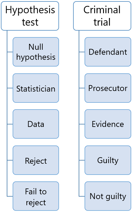
This process resembles a trial:
the defendant (the null hypothesis) is accused of being guilty (wrong);
evidence (data) is gathered in order to prove the defendant guilty (reject the null);
if there is evidence beyond any reasonable doubt, the defendant is found guilty (the null is rejected);
otherwise, the defendant is found not guilty (the null is not rejected).
Keep this analogy in mind because it helps to better understand statistical tests, their limitations, use and misuse, and frequent misinterpretation.
Before collecting the data:
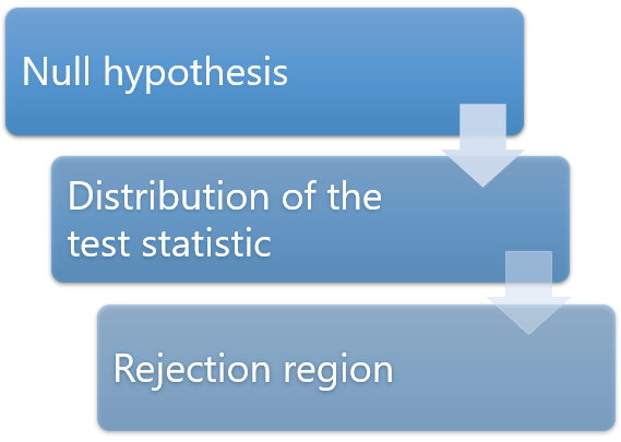
we decide how to summarize the relevant characteristics of the sample data in a single number, the so-called test statistic;
we derive the probability distribution of the test statistic under the hypothesis that the null is true (the data is regarded as random; therefore, the test statistic is a random variable);
we decide what probability of incorrectly rejecting the null we are willing to tolerate (the level of significance, or size of the test); the level of significance is typically a small number, such as 5% or 1%.
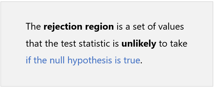
we choose one or more intervals of values (collectively called rejection region) such that the probability that the test statistic falls within these intervals is equal to the desired level of significance; the rejection region is often a tail of the distribution of the test statistic (one-tailed test) or the union of the left and right tails (two-tailed test).
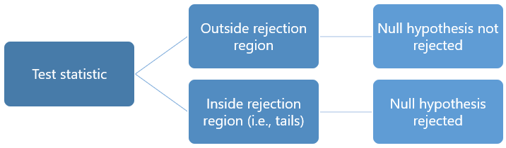
Then, the data is collected and used to compute the value of the test statistic.
A decision is taken as follows:
if the test statistic falls within the rejection region, then the null hypothesis is rejected;
otherwise, it is not rejected.
We now make two examples of practical problems that lead to formulate and test a null hypothesis.
A new method is proposed to produce light bulbs.
The proponents claim that it produces less defective bulbs than the method currently in use.
To check the claim, we can set up a statistical test as follows.
We keep the light bulbs on for 10 consecutive days, and then we record whether they are still working at the end of the test period.
The probability that a light bulb produced with the new method is still working at the end of the test period is the same as that of a light bulb produced with the old method.
100 light bulbs are tested:
50 of them are produced with the new method (group A)
the remaining 50 are produced with the old method (group B).
The final data comprises 100 observations of:
an indicator variable which is equal to 1 if the light bulb is still working at the end of the test period and 0 otherwise;
a categorical variable that records the group (A or B) to which each light bulb belongs.
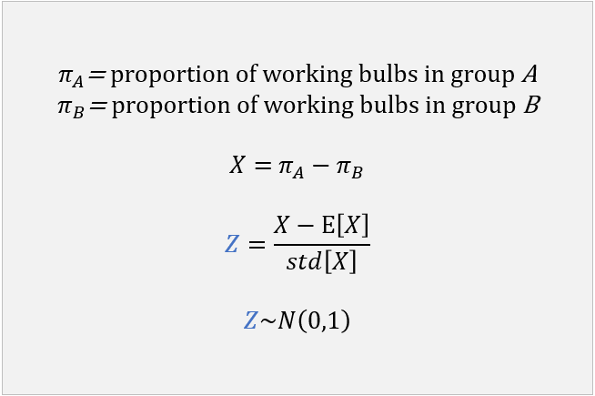
We use the data to compute the proportions of working light bulbs in groups A and B.
The proportions are estimates of the probabilities of not being defective, which are equal for the two groups under the null hypothesis.
We then compute a z-statistic (see here for details) by:
taking the difference between the proportion in group A and the proportion in group B;
standardizing the difference:
we subtract the expected value (which is zero under the null hypothesis);
we divide by the standard deviation (it can be derived analytically).
The distribution of the z-statistic can be approximated by a standard normal distribution.
We decide that the level of confidence must be 5%. In other words, we are going to tolerate a 5% probability of incorrectly rejecting the null hypothesis.
The critical region is the right 5%-tail of the normal distribution, that is, the set of all values greater than 1.645 (see the glossary entry on critical values if you are wondering how this value was obtained).
If the test statistic is greater than 1.645, then the null hypothesis is rejected; otherwise, it is not rejected.
A rejection is interpreted as significant evidence that the new production method produces less defective items; failure to reject is interpreted as insufficient evidence that the new method is better.
A production plant incurs high costs when production needs to be halted because some machinery fails.
The plant manager has decided that he is not willing to tolerate more than one halt per year on average.
If the expected number of halts per year is greater than 1, he will make new investments in order to improve the reliability of the plant.
A statistical test is set up as follows.
The reliability of the plant is measured by the number of halts.
The number of halts in a year is assumed to have a Poisson distribution with expected value equal to 1 (using the Poisson distribution is common in reliability testing).
The manager cannot wait more than one year before taking a decision.
There will be a single datum at his disposal: the number of halts observed during one year.
The number of halts is used as a test statistic. By assumption, it has a Poisson distribution under the null hypothesis.
The manager decides that the probability of incorrectly rejecting the null can be at most 10%.
A Poisson random variable with expected value equal to 1 takes values:
larger than 1 with probability 26.42%;
larger than 2 with probability 8.03%.
Therefore, it is decided that the critical region will be the set of all values greater than or equal to 3.
If the test statistic is strictly greater than or equal to 3, then the null is rejected; otherwise, it is not rejected.
A rejection is interpreted as significant evidence that the production plant is not reliable enough (the average number of halts per year is significantly larger than tolerated).
Failure to reject is interpreted as insufficient evidence that the plant is unreliable.
This section discusses the main problems that arise in the interpretation of the outcome of a statistical test (reject / not reject).
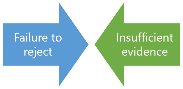
When the test statistic does not fall within the critical region, then we do not reject the null hypothesis.
Does this mean that we accept the null? Not really.
In general, failure to reject does not constitute, per se, strong evidence that the null hypothesis is true.
Remember the analogy between hypothesis testing and a criminal trial. In a trial, when the defendant is declared not guilty, this does not mean that the defendant is innocent. It only means that there was not enough evidence (not beyond any reasonable doubt) against the defendant.
In turn, lack of evidence can be due:
either to the fact that the defendant is innocent;
or to the fact that the prosecution has not been able to provide enough evidence against the defendant, even if the latter is guilty.
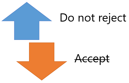
This is the very reason why courts do not declare defendants innocent, but they use the locution "not guilty".
In a similar fashion, statisticians do not say that the null hypothesis has been accepted, but they say that it has not been rejected.
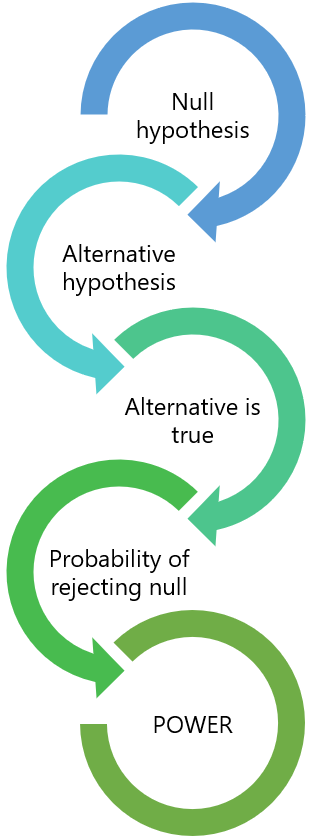
To better understand why failure to reject does not in general constitute strong evidence that the null hypothesis is true, we need to use the concept of statistical power.
The power of a test is the probability (calculated ex-ante, i.e., before observing the data) that the null will be rejected when another hypothesis (called the alternative hypothesis) is true.
Let's consider the first of the two examples above (the production of light bulbs).
In that example, the null hypothesis is: the probability that a light bulb is defective does not decrease after introducing a new production method.
Let's make the alternative hypothesis that the probability of being defective is 1% smaller after changing the production process (assume that a 1% decrease is considered a meaningful improvement by engineers).
How much is the ex-ante probability of rejecting the null if the alternative hypothesis is true?
If this probability (the power of the test) is small, then it is very likely that we will not reject the null even if it is wrong.
If we use the analogy with criminal trials, low power means that most likely the prosecution will not be able to provide sufficient evidence, even if the defendant is guilty.
Thus, in the case of lack of power, failure to reject is almost meaningless (it was anyway highly likely).
This is why, before performing a test, it is good statistical practice to compute its power against a relevant alternative.
If the power is found to be too small, there are usually remedies. In particular, statistical power can usually be increased by increasing the sample size (see, e.g., the lecture on hypothesis tests about the mean).
As we have explained above, interpreting a failure to reject the null hypothesis is not always straightforward. Instead, interpreting a rejection is somewhat easier.
When we reject the null, we know that the data has provided a lot of evidence against the null. In other words, it is unlikely (how unlikely depends on the size of the test) that the null is true given the data we have observed.
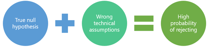
There is an important caveat though. The null hypothesis is often made up of several assumptions, including:
the main assumption (the one we are testing);
other assumptions (e.g., technical assumptions) that we need to make in order to set up the hypothesis test.
For instance, in Example 2 above (reliability of a production plant), the main assumption is that the expected number of production halts per year is equal to 1. But there is also a technical assumption: the number of production halts has a Poisson distribution.
It must be kept in mind that a rejection is always a joint rejection of the main assumption and all the other assumptions.
Therefore, we should always ask ourselves whether the null has been rejected because the main assumption is wrong or because the other assumptions are violated.
In the case of Example 2 above, is a rejection of the null due to the fact that the expected number of halts is greater than 1 or is it due to the fact that the distribution of the number of halts is very different from a Poisson distribution?
When we suspect that a rejection is due to the inappropriateness of some technical assumption (e.g., assuming a Poisson distribution in the example), we say that the rejection could be due to misspecification of the model.
The right thing to do when these kind of suspicions arise is to conduct so-called robustness checks, that is, to change the technical assumptions and carry out the test again.
In our example, we could re-run the test by assuming a different probability distribution for the number of halts (e.g., a negative binomial or a compound Poisson - do not worry if you have never heard about these distributions).
If we keep obtaining a rejection of the null even after changing the technical assumptions several times, the we say that our rejection is robust to several different specifications of the model.
What are the main practical implications of everything we have said thus far? How does the theory above help us to set up and test a null hypothesis?
What we said can be summarized in the following guiding principles:
A test of hypothesis is like a criminal trial and you are the prosecutor. You want to find evidence that the defendant (the null hypothesis) is guilty. Your job is not to prove that the defendant is innocent. If you find yourself hoping that the defendant is found not guilty (i.e., the null is not rejected) then something is wrong with the way you set up the test. Remember: you are the prosecutor.
Compute the power of your test against one or more relevant alternative hypotheses. Do not run a test if you know ex-ante that it is unlikely to reject the null when the alternative hypothesis is true.
Beware of technical assumptions that you add to the main assumption you want to test. Make robustness checks in order to verify that the outcome of the test is not biased by model misspecification.
The null hypothesis is usually denoted by the symbol
![]() (read "H-zero", "H-nought" or "H-null"). The letter
(read "H-zero", "H-nought" or "H-null"). The letter
![]() in the symbol stands for "Hypothesis".
in the symbol stands for "Hypothesis".
More examples of null hypotheses and how to test them can be found in the following lectures.
| Where the example is found | Null hypothesis |
|---|---|
| Hypothesis testing about the mean | The mean of a normal distribution is equal to a certain value |
| Hypothesis testing about the variance | The variance of a normal distribution is equal to a certain value |
| Hypothesis testing in maximum likelihood estimation | A vector of parameters estimated by MLE satisfies a set of linear or non-linear restrictions |
| Hypothesis testing in linear regression models | A regression coefficient is equal to a certain value |
The lecture on Hypothesis testing provides a more detailed mathematical treatment of null hypotheses and how they are tested.
This lecture on the null hypothesis was featured in Stanford University's Best practices in science.

Previous entry: Normal equations
Next entry: Parameter
Please cite as:
Taboga, Marco (2021). "Null hypothesis", Lectures on probability theory and mathematical statistics. Kindle Direct Publishing. Online appendix. https://www.statlect.com/glossary/null-hypothesis.
Most of the learning materials found on this website are now available in a traditional textbook format.