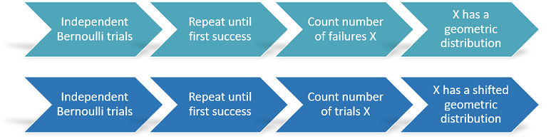
The geometric distribution is the probability distribution of the number of failures we get by repeating a Bernoulli experiment until we obtain the first success.
![]()
Consider a Bernoulli experiment, that is, a random experiment having two possible outcomes: either success or failure.
We repeat the experiment until we get the first success, and then we count the
number
![]() of failures that we faced prior to recording the success.
of failures that we faced prior to recording the success.
Since the experiments are random,
![]() is a random
variable.
is a random
variable.
If the repetitions of the experiment are
independent
of each other, then the distribution of
![]() is called geometric distribution.
is called geometric distribution.
Example If we toss a coin until we obtain head, the number of tails before the first head has a geometric distribution.
At the end of this lecture we will also study a slight variant of the geometric distribution, called shifted geometric distribution. The latter is the distribution of the total number of trials (all the failures + the first success).
In other words, if
![]() has a geometric distribution, then
has a geometric distribution, then
![]() has a shifted geometric distribution.
has a shifted geometric distribution.
The geometric distribution is characterized as follows.
Definition
Let
![]() be a discrete random
variable. Let
be a discrete random
variable. Let
![]() .
Let the support of
.
Let the support of
![]() be the set of non-negative
integers
be the set of non-negative
integers![]() We
say that
We
say that
![]() has a geometric distribution with
parameter
has a geometric distribution with
parameter
![]() if its probability mass
function
is
if its probability mass
function
is![[eq3]](/images/geometric-distribution__12.png)
The following is a proof that
![]() is a legitimate probability mass function.
is a legitimate probability mass function.
The probabilities
![]() are well-defined and non-negative for any
are well-defined and non-negative for any
![]() because
because
![]() .
We just need to prove that the sum of
.
We just need to prove that the sum of
![]() over its support equals
over its support equals
![]() :
:
![[eq8]](data:image/gif;base64,R0lGODlhAQABAIAAANvf7wAAACH5BAEAAAAALAAAAAABAAEAAAICRAEAOw==) where
in step
where
in step
![]() we have used the
formula for
geometric series.
we have used the
formula for
geometric series.
Remember that a Bernoulli random variable is equal to:
![]() (success) with probability
(success) with probability
![]() ;
;
![]() (failure) with probability
(failure) with probability
![]() .
.
The following proposition shows how the geometric distribution is related to the Bernoulli distribution.
Proposition
Let
![]() be a sequence of independent Bernoulli random variables with parameter
be a sequence of independent Bernoulli random variables with parameter
![]() .
Then, for any integer
.
Then, for any integer
![]() ,
the probability that
,
the probability that
![]() for
for
![]() and
and
![]() is
is![]() where
where
![]() is the probability mass function of a geometric distribution with parameter
is the probability mass function of a geometric distribution with parameter
![]() .
.
Since the Bernoulli random variables are
independent, we have
that![[eq12]](/images/geometric-distribution__34.png)
The expected value of a geometric random variable
![]() is
is
It can be derived as
follows:![[eq14]](/images/geometric-distribution__37.png)
The variance of a geometric random variable
![]() is
is
Let us first derive the
second moment of
![]() :
:![[eq16]](/images/geometric-distribution__41.png) Now,
we can use the variance
formula:
Now,
we can use the variance
formula:![[eq17]](/images/geometric-distribution__42.png)
The moment generating function of a
geometric random variable
![]() is defined for any
is defined for any
![]() :
:
This is proved as
follows:where
the series in step
![]() converges only if
converges only if
![]() that
is, only
ifBy
taking the natural log of both sides, the condition
becomes
that
is, only
ifBy
taking the natural log of both sides, the condition
becomes![]()
The characteristic function of a geometric random
variable
![]() is
is![[eq24]](/images/geometric-distribution__52.png)
The proof is similar to the proof for the
mgf:
The distribution function
of a geometric random variable
![]() is
is![[eq26]](/images/geometric-distribution__55.png)
For
![]() ,
,
![]() ,
because
,
because
![]() cannot be smaller than
cannot be smaller than
![]() .
For
.
For
![]() ,
we
have
,
we
have
As we have said in the introduction, the geometric distribution is the distribution of the number of failed trials before the first success.
The shifted geometric distribution is the distribution of the total number of trials (all the failures + the first success).
In other words, if
![]() has a geometric distribution, then
has a geometric distribution, then
![]() has
a shifted geometric distribution.
has
a shifted geometric distribution.
It is then simple to derive the properties of the shifted geometric distribution.
It expected value
is
Its variance
is
Its moment generating function is, for any
![]() :
:
Its characteristic function
is![[eq34]](/images/geometric-distribution__68.png)
Its distribution function
is
The geometric distribution is considered a discrete version of the exponential distribution.
Suppose that the Bernoulli experiments are performed at equal time intervals.
Then, the geometric random variable
![]() is the time (measured in discrete units) that passes before
we obtain the first success.
is the time (measured in discrete units) that passes before
we obtain the first success.
Contrast this with the fact that the exponential distribution is used to model the time elapsed before a given event occurs when time is continuous.
From a mathematical viewpoint, the geometric distribution enjoys the same memoryless property possessed by the exponential distribution:
in the exponential case, the probability that the event happens during a given time interval is independent of how much time has already passed without the event happening;
in the geometric case, the probability that the event happens at a given point in (discrete) time is not dependent on what happened before; in fact, the Bernoulli experiment performed at each point in time is independent of previous trials.
Below you can find some exercises with explained solutions.
On each day we play a lottery in which the probability of winning is
![]() .
.
What is the expected value of the number of days that will elapse before we win for the first time?
Each time we play the lottery, the
outcome is a Bernoulli random variable (equal to 1 if we win), with parameter
![]() .
Therefore, the number of days before winning is a geometric random variable
with parameter
.
Therefore, the number of days before winning is a geometric random variable
with parameter
![]() .
Its expected value
is
.
Its expected value
is
Please cite as:
Taboga, Marco (2021). "Geometric distribution", Lectures on probability theory and mathematical statistics. Kindle Direct Publishing. Online appendix. https://www.statlect.com/probability-distributions/geometric-distribution.
Most of the learning materials found on this website are now available in a traditional textbook format.