Gauss Jordan elimination algorithm

Gauss Jordan elimination is an algorithm that allows us to transform a linear system into an equivalent system in reduced row echelon form.

The main difference with respect to Gaussian elimination is illustrated by the following diagram.

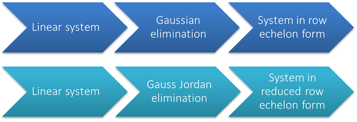
A diagram illustrating the differences between the Gaussian and Gauss Jordan elimination algorithms

In this lecture we are going to assume that the reader is already familiar with Gaussian elimination and aware of the differences between row echelon form and reduced row echelon form.

Table of contents

Overview
Steps of the algorithm
Examples
Gauss Jordan elimination with pivoting
Solved exercises
1. Exercise 1

Overview

The aim of the Gauss Jordan elimination algorithm is to transform a linear system of equations in unknowns [eq1] into an equivalent system (i.e., a system having the same solutions) in reduced row echelon form.

The system can be written aswhere is the coefficient matrix, is the vector of unknowns and is a constant vector.

Remember that a system is in reduced row echelon form if its coefficient matrix has the following properties:

all non-zero rows contain an element, called pivot, that is non-zero and has only zero entries below it and to its left;
all pivots are equal to ;
a pivot is the only non-zero element of its column;
zero-rows (if there are any) are below the non-zero rows;

Gauss Jordan elimination consists in a sequence of elementary row operations:

interchanging the order of the equations, so as to make sure that the zero rows are at the bottom of the matrix;
multiplying (or dividing) the equations by non-zero constants, so as to make the pivots equal to ;
adding multiples of some equations to other equations, so as to annihilate the entries above and below the pivots.

Steps of the algorithm

The Gauss Jordan algorithm is very similar to Gaussian elimination. Therefore, we are not going to explain its steps in detail, but we are only going to comment on the differences with respect to Gaussian elimination. Please refer to the lecture on Gaussian elimination for detailed explanations.

Before laying out the algorithm, we warn the reader that the coefficient matrix of the system will be denoted by both before and after performing an elementary row operation, even if the matrix resulting from the operation is in principle a different matrix.

The steps are listed below:

Start from and .
Increment by one unit.
Increment by one unit.
Stop the algorithm if . Else proceed to the next step.
If $A_{il}=0$ for , return to step 3. Else proceed to the next step.
Interchange the -th equation with any equation (with ) such that $A_{il} eq 0$ (if there is no need to perform an interchange).
Divide the -th equation by $A_{kl}$ .
For and , subtract the -th equation multiplied by $A_{il}$ from the -th equation.
If , return to step 2. Else stop the algorithm.

The differences with respect to Gaussian elimination are the following:

Step 7 is not found in the Gaussian elimination algorithm. In step 7, we divide the equation containing the current pivot by the value of the pivot itself. This is done to ensure that all pivots are equal to in the final system.
In step 8, we perform elementary operations to annihilate not only the elements below the pivot (as in Gaussian elimination) but also those above it.
In step 9, we stop at the last row, unlike in Gaussian elimination, where we stop at the penultimate row. The reason is that, if there is a pivot on the last row, we need to make it equal to , and we need to annihilate the entries above it.

Examples

We present below an example of Gauss Jordan elimination.

In order to simplify the notation, we are going to use augmented matrices to represent linear systems.

Example Consider the system of three equations in four unknowns represented by the augmented matrix [eq3] We start from row and column . Since , we do not perform any interchange of rows. We divide the first row by $A_{11}=-1$ and obtain [eq5] In order to annihilate the entries below the pivot $A_{11}$ , we subtract the first row multiplied by from the second and multiplied by from the third: [eq6] We move to row and column . Since $A_{kl}=A_{22}=0$ , but $A_{32} eq 0$ , we interchange the second row with the third: [eq7] We divide the second row by $A_{22}=2$ : [eq8] We add the second row multiplied by to the first: [eq9] We move to row and column . We divide the third row by the value of its pivot $A_{33}=18$ : [eq10] We add times the third row to the second and the third: [eq11] The matrix is now in reduced row echelon form.

Gauss Jordan elimination with pivoting

As in Gaussian elimination, in order to improve the numerical stability of the algorithm, we usually perform partial pivoting in step 6, that is, we always choose the row interchange that moves the largest element (in absolute value) to the pivotal position. If we also exchange columns in order to maximize the absolute value of the pivot, then we are doing complete pivoting. See the lecture on Gaussian elimination for more details on partial and complete pivoting.

Solved exercises

Below you can find some exercises with explained solutions.

Exercise 1

Transform the system [eq12] into an equivalent system in reduced row echelon form. Use the Gauss Jordan elimination algorithm with partial pivoting.

Solution

The entry $A_{11}$ is non-zero and it is already the largest entry in the first column. Therefore, it is used as pivot. Divide the first row by $A_{11}=2$ : [eq13] Annihilate the entries below the pivot $A_{11}$ : [eq14] Interchange the second row with the third, so that the largest element moves to the pivotal position: [eq15] Divide the second row by $A_{22}=5/2$ : [eq16] Annihilate the entries above and below the pivot $A_{22}$ : [eq17] Interchange the third row with the fourth: [eq18] Divide the third row by $A_{33}=7$ : [eq19] All the elements above and below the pivot $A_{33}$ are already zero, so we can move to the last row. There are no row interchanges to consider because there are no rows below the last. Furthermore, $A_{44}$ is a pivot and it is already equal to . Therefore, we only need to annihilate the elements above it: [eq20] The system is now in reduced row echelon form.

How to cite

Please cite as:

Taboga, Marco (2021). "Gauss Jordan elimination algorithm", Lectures on matrix algebra. https://www.statlect.com/matrix-algebra/Gauss-Jordan-elimination.