The normal distribution is a continuous probability distribution that plays a central role in probability theory and statistics.
It is often called Gaussian distribution, in honor of Carl Friedrich Gauss (1777-1855), an eminent German mathematician who gave important contributions towards a better understanding of the normal distribution.
![]()
Table of contents
The normal distribution is extremely important because:
many real-world phenomena involve random quantities that are approximately normal (e.g., errors in scientific measurement);
it plays a crucial role in the Central Limit Theorem, one of the fundamental results in statistics;
its great analytical tractability makes it very popular in statistical modelling.
Sometimes it is also referred to as "bell-shaped distribution" because the graph of its probability density function resembles the shape of a bell.
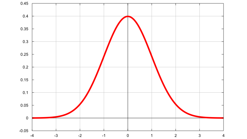
As you can see from the above plot, the density of a normal distribution has two main characteristics:
it is symmetric around the mean (indicated by the vertical line); as a consequence, deviations from the mean having the same magnitude, but different signs, have the same probability;
it is concentrated around the mean; it becomes smaller by moving from the center to the left or to the right of the distribution (the so called "tails" of the distribution); this means that the further a value is from the center of the distribution, the less probable it is to observe that value.
The remainder of this lecture gives a formal presentation of the main characteristics of the normal distribution.
First, we deal with the special case in which the distribution has zero mean and unit variance. Then, we present the general case, in which mean and variance can take any value.
The adjective "standard" indicates the special case in which the mean is equal to zero and the variance is equal to one.
Standard normal random variables are characterized as follows.
Definition
Let
![]() be a continuous
random variable. Let its
support be the whole
set of real
numbers:
be a continuous
random variable. Let its
support be the whole
set of real
numbers:![]() We
say that
We
say that
![]() has a standard normal distribution if and only if its
probability density function
is
has a standard normal distribution if and only if its
probability density function
is![[eq2]](data:image/gif;base64,R0lGODlhAQABAIAAANvf7wAAACH5BAEAAAAALAAAAAABAAEAAAICRAEAOw==)
The following is a proof that
![]() is indeed a legitimate probability density
function:
is indeed a legitimate probability density
function:
The function
![]() is a legitimate probability density function if it is non-negative and if its
integral over the support equals 1. The former property is obvious, while the
latter can be proved as
follows:
is a legitimate probability density function if it is non-negative and if its
integral over the support equals 1. The former property is obvious, while the
latter can be proved as
follows:
The expected value of a standard normal random
variable
![]() is
is![]()
It
can be derived as
follows:
The variance of a standard normal random variable
![]() is
is![]()
It
can be proved with the usual
variance formula
(![]() ):
):![[eq10]](/images/normal-distribution__14.png)
The moment generating function of a standard
normal random variable
![]() is defined for any
is defined for any
![]() :
:![]()
It
is derived by using the definition of moment generating
function:![[eq12]](/images/normal-distribution__18.png) The
integral above is well-defined and finite for any
The
integral above is well-defined and finite for any
![]() .
Thus, the moment generating function of
.
Thus, the moment generating function of
![]() exists for any
exists for any
![]() .
.
The characteristic function of a standard normal
random variable
![]() is
is![]()
By
the definition of characteristic function, we
haveNow,
take the derivative with respect to
![]() of the characteristic
function:
of the characteristic
function:![[eq15]](/images/normal-distribution__26.png) By
putting together the previous two results, we
obtain
By
putting together the previous two results, we
obtain![]() The
only function that satisfies this ordinary differential equation (subject to
the condition
The
only function that satisfies this ordinary differential equation (subject to
the condition
![]() )
is
)
is![]()
There is no simple formula for the
distribution function
![]() of a standard normal random variable
of a standard normal random variable
![]() because the
integral
because the
integral![]() cannot
be expressed in terms of elementary functions. Therefore, it is usually
necessary to resort to special tables or computer algorithms to compute the
values of
cannot
be expressed in terms of elementary functions. Therefore, it is usually
necessary to resort to special tables or computer algorithms to compute the
values of
![]() .
The lecture entitled Normal
distribution values discusses these alternatives in detail.
.
The lecture entitled Normal
distribution values discusses these alternatives in detail.
While in the previous section we restricted our attention to the special case of zero mean and unit variance, we now deal with the general case.
The normal distribution with mean
![]() and variance
and variance
![]() is characterized as follows.
is characterized as follows.
Definition
Let
![]() be a continuous random variable. Let its support be the whole set of real
numbers:
be a continuous random variable. Let its support be the whole set of real
numbers:![]() Let
Let
![]() and
and
![]() .
We say that
.
We say that
![]() has a normal distribution with mean
has a normal distribution with mean
![]() and variance
and variance
![]() if and only if its probability density function
is
if and only if its probability density function
is
We often indicate the fact that
![]() has a normal distribution with mean
has a normal distribution with mean
![]() and variance
and variance
![]() by
by![]()
To better understand how the shape of the distribution depends on its parameters, you can have a look at the density plots at the bottom of this page.
The following proposition provides the link between the standard and the general case.
Proposition
If
![]() has a normal distribution with mean
has a normal distribution with mean
![]() and variance
and variance
![]() ,
then
,
then![]() where
where
![]() is a random variable having a standard normal distribution.
is a random variable having a standard normal distribution.
This can be easily proved using the formula
for the density of a function of a
continuous variable
(![]() is a strictly increasing function of
is a strictly increasing function of
![]() ,
since
,
since
![]() is strictly
positive):
is strictly
positive):
Thus, a normal distribution is standard when
![]() and
and
![]() .
.
The expected value of a normal random variable
![]() is
is![]()
The
proof is a straightforward application of the fact that
![]() can we written as a linear function of a standard normal
variable:
can we written as a linear function of a standard normal
variable:
The variance of a normal random variable
![]() is
is![]()
It
can be derived as
follows:
The moment generating function of a normal random variable
![]() is defined for any
is defined for any
![]() :
:![]()
The
mgf is derived as
follows:![[eq34]](/images/normal-distribution__69.png) It
is defined for any
It
is defined for any
![]() because the moment generating function of
because the moment generating function of
![]() is defined for any
is defined for any
![]() .
.
The characteristic function of a normal random variable
![]() is
is![]()
The
derivation is similar to the derivation of the moment generating
function:![[eq36]](/images/normal-distribution__75.png)
The distribution function
![]() of a normal random variable
of a normal random variable
![]() can be written
as
can be written
as![]() where
where
![]() is the distribution function of a standard normal random variable
is the distribution function of a standard normal random variable
![]() (see above). The lecture entitled
Normal distribution values
provides a proof of this formula and discusses it in detail.
(see above). The lecture entitled
Normal distribution values
provides a proof of this formula and discusses it in detail.
This section shows the plots of the densities of some normal random variables. These plots help us to understand how the shape of the distribution changes by changing its parameters.
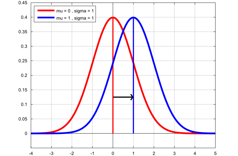
The following plot contains the graphs of two normal probability density functions:
the first graph (red line) is the probability density function of a normal
random variable with mean
![]() and standard deviation
and standard deviation
![]() ;
;
the second graph (blue line) is the probability density function of a normal
random variable with mean
![]() and standard deviation
and standard deviation
![]() .
.
By changing the mean from
![]() to
to
![]() ,
the shape of the graph does not change, but the graph is translated to the
right (its location changes).
,
the shape of the graph does not change, but the graph is translated to the
right (its location changes).
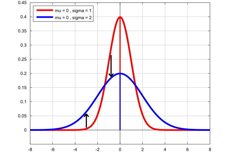
The following plot shows two graphs:
the first graph (red line) is the probability density function of a normal
random variable with mean
![]() and standard deviation
and standard deviation
![]() ;
;
the second graph (blue line) is the probability density function of a normal
random variable with mean
![]() and standard deviation
and standard deviation
![]() .
.
By increasing the standard deviation from
![]() to
to
![]() ,
the location of the graph does not change (it remains centered at
,
the location of the graph does not change (it remains centered at
![]() ),
but the shape of the graph changes (there is less density in the center and
more density in the tails).
),
but the shape of the graph changes (there is less density in the center and
more density in the tails).
The following lectures contain more material about the normal distribution.
How to tackle the numerical computation of the distribution function
Multivariate normal distribution
A multivariate generalization of the normal distribution, frequently encountered in statistics
Quadratic forms involving normal variables
Discusses the distribution of quadratic forms involving normal random variables
Linear combinations of normal variables
Discusses the important fact that normality is preserved by linear combinations
Below you can find some exercises with explained solutions.
Let
![]() be a normal random variable with mean
be a normal random variable with mean
![]() and variance
and variance
![]() .
Compute the following
probability:
.
Compute the following
probability:![]()
First of all, we need to express the
above probability in terms of the distribution function of
![]() :
:![[eq41]](/images/normal-distribution__99.png)
Then, we need to express the distribution function of
![]() in terms of the distribution function of a standard normal random variable
in terms of the distribution function of a standard normal random variable
![]() :
:![]()
Therefore, the above probability can be expressed
aswhere
we have used the fact that
![]() ,
which has been presented in the lecture entitled
Normal distribution values.
,
which has been presented in the lecture entitled
Normal distribution values.
Let
![]() be a random variable having a normal distribution with mean
be a random variable having a normal distribution with mean
![]() and variance
and variance
![]() .
Compute the following
probability:
.
Compute the following
probability:![]()
We need to use the same technique used in
the previous exercise (express the probability in terms of the distribution
function of a standard normal random
variable):where
we have found the value
![]() in a normal distribution table.
in a normal distribution table.
Suppose the random variable
![]() has a normal distribution with mean
has a normal distribution with mean
![]() and variance
and variance
![]() .
Define the random variable
.
Define the random variable
![]() as
follows:
as
follows:![]() Compute
the expected value of
Compute
the expected value of
![]() .
.
Remember that the moment generating
function of
![]() isTherefore,
using the linearity of the expected value, we
obtain
isTherefore,
using the linearity of the expected value, we
obtain
Please cite as:
Taboga, Marco (2021). "Normal distribution", Lectures on probability theory and mathematical statistics. Kindle Direct Publishing. Online appendix. https://www.statlect.com/probability-distributions/normal-distribution.
Most of the learning materials found on this website are now available in a traditional textbook format.