In statistics and machine learning, a loss function quantifies the losses generated by the errors that we commit when:
we estimate the parameters of a statistical model;
we use a predictive model, such as a linear regression, to predict a variable.
The minimization of the expected loss, called statistical risk, is one of the guiding principles in statistical modelling.
![]()
Table of contents
In order to introduce loss functions, we use the example of a
linear regression
model![]() where
where
![]() is the dependent variable,
is the dependent variable,
![]() is a vector of regressors,
is a vector of regressors,
![]() is a vector of regression coefficients and
is a vector of regression coefficients and
![]() is an unobservable error term.
is an unobservable error term.
Suppose that we use some data to produce an estimate
![]() of the unknown vector
of the unknown vector
![]() .
.
In general, there is a non-zero
difference![]() between
our estimate and the true value, called estimation error.
between
our estimate and the true value, called estimation error.
Of course, we would like estimation errors to be as small as possible. But how do we formalize this preference?
We use a
function![]() that
quantifies the losses incurred because of the estimation error, by mapping
couples
that
quantifies the losses incurred because of the estimation error, by mapping
couples
![]() to the set of real numbers.
to the set of real numbers.
Typically, loss functions are increasing in the absolute value of the estimation error and they have convenient mathematical properties, such as differentiability and convexity.
An example (when
![]() is a scalar) is the quadratic
loss
is a scalar) is the quadratic
loss![]()
After we have estimated a linear regression model, we can compare its predictions of the dependent variable to the true values.
Given the regressors
![]() ,
the prediction of
,
the prediction of
![]() is
is![]()
The
difference![]() between
the prediction and the true value is called prediction error.
between
the prediction and the true value is called prediction error.
As in the case of estimation errors, we have a preference for small prediction
errors. We formalize it by specifying a loss
function![]() that
maps couples
that
maps couples
![]() to real numbers.
to real numbers.
Most of the functions that are used to quantify prediction losses are also used for estimation losses.
The expected value of the loss is called risk.
When
![]() is seen as an estimator (i.e., a random
variable whose realization is equal to the estimate), the expected
value
is seen as an estimator (i.e., a random
variable whose realization is equal to the estimate), the expected
value![]() is
the risk of the estimator.
is
the risk of the estimator.
The other relevant quantity is the risk of the
predictions![]() which
can be approximated by the empirical risk, its sample
counterpart:
which
can be approximated by the empirical risk, its sample
counterpart:![[eq12]](data:image/gif;base64,R0lGODlhAQABAIAAANvf7wAAACH5BAEAAAAALAAAAAABAAEAAAICRAEAOw==) where
where
![]() is the sample size.
is the sample size.
In a linear regression model, the vector of regression coefficients is usually estimated by empirical risk minimization.
The predictions
![]() depend on
depend on
![]() and so does the empirical risk. We search for a vector
and so does the empirical risk. We search for a vector
![]() that minimizes the empirical risk.
that minimizes the empirical risk.
The Ordinary
Least Squares (OLS) estimator of
![]() is the empirical risk minimizer when the quadratic loss (details below) is
used as the loss function.
is the empirical risk minimizer when the quadratic loss (details below) is
used as the loss function.
In fact, the OLS estimator solves the minimization
problem![[eq13]](/images/loss-function__28.png)
Under the conditions stated in the Gauss-Markov theorem, the OLS estimator is also the unbiased estimator that generates the lowest expected estimation losses, provided that the quadratic loss is used to quantify the latter.
What we have said thus far regarding linear regressions applies more in general to:
all statistical models (as far as estimation losses are concerned);
all predictive models (as far as prediction losses are concerned).
In other words, given a parametric statistical model, we can always define a loss function that depends on parameter estimates and true parameter values.
Given a predictive model, we can use a loss function to compare predictions to observed values.
We now introduce some common loss function.
We will always use the
![]() notation, but most of the functions we present can be used both in estimation
and in prediction.
notation, but most of the functions we present can be used both in estimation
and in prediction.
It is important to note that we can always multiply a loss function by a positive constant and/or add an arbitrary constant to it. These transformations do not change model rankings and the results of empirical risk minimization. In fact, the solution to an optimization problem does not change when the said transformations are performed on the objective function.
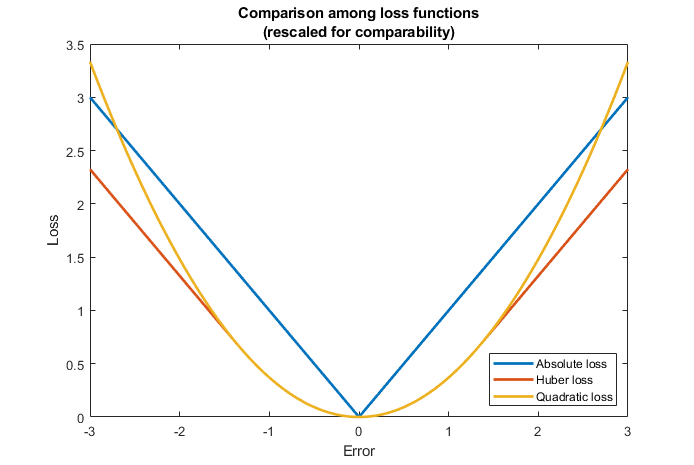
The most popular loss function is the quadratic loss (or squared error, or L2 loss).
When
![]() is a scalar, the quadratic loss
is
is a scalar, the quadratic loss
is![]()
When
![]() is a vector, it is defined
as
is a vector, it is defined
as![]() where
where
![]() denotes
the Euclidean norm.
denotes
the Euclidean norm.
When the loss is quadratic, the expected value of the loss (the risk) is called Mean Squared Error (MSE).
The quadratic loss is immensely popular because it often allows us to derive closed-form expressions for the parameters that minimize the empirical risk and for the expected loss. This is exactly what happens in the linear regression model discussed above.
Squaring the prediction errors creates strong incentives to reduce very large errors, possibly at the cost of significantly increasing smaller ones.
For example, according to the quadratic loss function, Configuration 2 below
is better than Configuration 1: we accept a large increase in
![]() (by 3 units) in order to obtain a small decrease in
(by 3 units) in order to obtain a small decrease in
![]() (by 1 unit).
(by 1 unit).
![[eq20]](/images/loss-function__37.png)
This kind of behavior makes the quadratic loss non-robust to outliers.
The absolute loss (or absolute error, or L1 loss) is defined
as![]() when
when
![]() is a scalar and as
is a scalar and as
![]() when
when
![]() is a vector.
is a vector.
When the loss is absolute, the expected value of the loss (the risk) is called Mean Absolute Error (MAE).
Unlike the quadratic loss, the absolute loss does not create particular incentives to reduce large errors, as only the average magnitude matters.
For example, according to the absolute loss, we should be indifferent between
Configuration 1 and 2 below. An increase in the magnitude of a large error is
acceptable if it is compensated by an equal decrease in an already small
error.
![[eq23]](/images/loss-function__42.png)
The absolute loss has the advantage of being more robust to outliers than the quadratic loss.
However, the absolute loss does not enjoy the same analytical tractability of the quadratic loss.
For instance, when we use the absolute loss in linear regression modelling, and we estimate the regression coefficients by empirical risk minimization, the minimization problem does not have a closed-form solution. This kind of approach is called Least Absolute Deviation (LAD) regression. You can read more details about it on Wikipedia.
The Huber loss is defined
as![[eq24]](/images/loss-function__43.png) where
where
![]() is a positive real number
chosen
by the statistician (if the errors are expected to be approximately
standard normal,
but there are some outliers,
is a positive real number
chosen
by the statistician (if the errors are expected to be approximately
standard normal,
but there are some outliers,
![]() is often deemed a good choice).
is often deemed a good choice).
Thus, the Huber loss blends the quadratic function, which applies to the
errors below the threshold
![]() ,
and the absolute function, which applies to the errors above
,
and the absolute function, which applies to the errors above
![]() .
.
In a sense, it tries to put together the best of both worlds (L1 and L2). Indeed, empirical risk minimization with the Huber loss function is optimal from several mathematical point of views in linear regressions contaminated by outliers.
There are several other loss functions commonly used in linear regression problems. For example:
the log-cosh
loss![]() which
is very similar to the Huber function, but unlike the latter is twice
differentiable everywhere;
which
is very similar to the Huber function, but unlike the latter is twice
differentiable everywhere;
the pseudo-Huber
loss![[eq26]](/images/loss-function__49.png) which
also behaves like the L2 loss near
zero and like the L1 loss elsewhere;
which
also behaves like the L2 loss near
zero and like the L1 loss elsewhere;
the epsilon-insensitive
loss![]() where
where
![]() is a threshold below which errors are ignored (treated as if they were zero);
the intuitive idea is that a very small error is as good as no error.
is a threshold below which errors are ignored (treated as if they were zero);
the intuitive idea is that a very small error is as good as no error.
Other loss functions are used in
classification
models, that is, in models in which the dependent variable
![]() is categorical (binary or multinomial).
is categorical (binary or multinomial).
The most important are:
the log-loss (or
cross-entropy)![[eq28]](/images/loss-function__53.png) where
where
![]() is a
is a
![]() multinoulli
vector (when the true category is the
multinoulli
vector (when the true category is the
![]() -th,
then
-th,
then
![]() and all the other entries of the vector
and all the other entries of the vector
![]() are zero), and
are zero), and
![]() is a vector of predictions;
is a vector of predictions;
the hinge loss (or margin
loss)![]() which
can be used when the variable
which
can be used when the variable
![]() can take only two values
(
can take only two values
(![]() or
or
![]() ).
).
More details about loss functions, estimation errors and statistical risk can be found in the lectures on Point estimation and Predictive models.
Previous entry: Log likelihood
Next entry: Marginal distribution function
Please cite as:
Taboga, Marco (2021). "Loss function", Lectures on probability theory and mathematical statistics. Kindle Direct Publishing. Online appendix. https://www.statlect.com/glossary/loss-function.
Most of the learning materials found on this website are now available in a traditional textbook format.