What is the probability that the realization of a random variable will be less than or equal to a certain threshold value?
The distribution function of a random variable allows us to answer exactly this question.
Its value at a given point is equal to the probability of observing a realization of the random variable below that point or equal to that point.
![]()
The distribution function is also often called cumulative distribution function (abbreviated as cdf).
The following is a formal definition.
Definition
If
![]() is a random variable, its distribution function is a function
is a random variable, its distribution function is a function
![]() such
that
such
that![]() where
where
![]() is the probability
that
is the probability
that
![]() is less than or equal to
is less than or equal to
![]() .
.
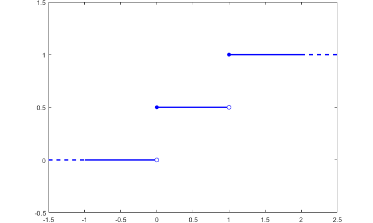
Suppose that a random variable can take only two values (0 and 1), each with probability 1/2.
Its distribution function
is![[eq4]](/images/distribution-function__7.png)
Here is a plot of the function.
Every distribution function enjoys the following four properties:
Increasing.
![]() is increasing, i.e.,
is increasing, i.e.,
![]()
Right-continuous.
![]() is right-continuous,
i.e.,
is right-continuous,
i.e.,![[eq8]](data:image/gif;base64,R0lGODlhAQABAIAAANvf7wAAACH5BAEAAAAALAAAAAABAAEAAAICRAEAOw==) for
any
for
any
![]() ;
;
Limit at minus infinity.
![]() satisfies
satisfies
![]()
Limit at plus infinity.
![]() satisfies
satisfies
![]()
Concise proofs of these properties can be found here and in Williams (1991).
Any distribution function enjoys the four properties above.
Moreover, for any given function enjoying these four properties, it is possible to define a random variable that has the given function as its distribution function (for a proof, see Williams 1991, Sec. 3.11).
The practical consequence of this fact is that, when we need to check whether a given function is a proper distribution function, we just need to verify that it satisfies the four properties above.
When the random variable
![]() is discrete, the cdf can be
derived
aswhere:
is discrete, the cdf can be
derived
aswhere:
![]() is the support of
is the support of
![]() ;
;
![]() is the probability mass
function of
is the probability mass
function of
![]() .
.
This can be quickly done with a table.
Suppose that the probability mass function of
![]() is
is![[eq15]](/images/distribution-function__24.png)
Then, we can set up a table that has three rows.
In the first row, we write the possible values of
![]() ,
sorted from smallest to largest.
,
sorted from smallest to largest.
In the second row, we write the probabilities of the single values.
The third row contains the values of the cdf.
The leftmost cell in the third row is equal to the cell immediately above.
Then, we go from left to right and the value in each cell is set equal to the sum of:
the probability in the cell immediately to the left;
the probability in the cell immediately above.
![[eq16]](/images/distribution-function__26.png)
Thus, the distribution function
is![[eq17]](/images/distribution-function__27.png)
When the random variable is
continuous, its
cdf can be computed
as![]() where
where
![]() is the probability density
function of
is the probability density
function of
![]() .
.
The simplest example is probably the cdf of the uniform distribution.
The probability density function of a random variable having uniform
distribution on the interval
![]() is
is![]() where
where
![]() is an indicator function that takes value 1 on the interval
is an indicator function that takes value 1 on the interval
![]() and value 0 everywhere else.
and value 0 everywhere else.
There are three cases:
if
![]() ,
then
,
then![]()
if
![]() ,
then
,
then![]()
if
![]() ,
then
,
then![]()
Therefore, the cdf
is![[eq26]](/images/distribution-function__41.png)
More details about the distribution function can be found in the lecture on Random variables.
Williams, D., 1991. Probability with martingales. Cambridge university press.
Previous entry: Discrete random vector
Next entry: Estimator
Please cite as:
Taboga, Marco (2021). "Distribution function", Lectures on probability theory and mathematical statistics. Kindle Direct Publishing. Online appendix. https://www.statlect.com/glossary/distribution-function.
Most of the learning materials found on this website are now available in a traditional textbook format.