In this lecture we introduce and discuss the notion of quantile of the probability distribution of a random variable.
At the end of the lecture, we report some quantiles of the normal distribution, which are often used in hypothesis testing.
![]()
We start with an informal definition.
The
![]() -quantile
of a random
variable
-quantile
of a random
variable
![]() is a value, denoted by
is a value, denoted by
![]() ,
such that:
,
such that:
![]()
![]() with probability
with probability
![]() ;
;
![]()
![]() with probability
with probability
![]() .
.
Thus, the quantile
![]() is a cut-off point that divides the
support of
is a cut-off point that divides the
support of
![]() in two parts:
in two parts:
the part to the left of
![]() ,
which has probability
,
which has probability
![]() ;
;
the part to the right of
![]() ,
which has probability
,
which has probability
![]() .
.
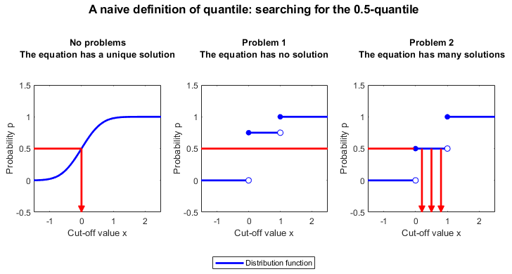
There are important cases in which the informal definition works perfectly well. However, there are also many cases in which it is flawed. Let us see why.
In the above definition, we require
that![]()
Remember that the distribution
function
![]() of a random variable
of a random variable
![]() is defined
as
is defined
as![]()
Therefore, we are asking
that![]()
However, we know that the distribution function may be discontinuous. In other
words, it may jump and it may not take all the values between
![]() and
and
![]() .
.
As a consequence, there may not exist a value
![]() that satisfies equation (1). The distribution function may jump from a value
lower than
that satisfies equation (1). The distribution function may jump from a value
lower than
![]() to a value higher than
to a value higher than
![]() without ever being equal to
without ever being equal to
![]() .
.
The lack of existence of a solution to equation (1) is not the only problem.
In fact, not only the distribution function may jump, but it may also be flat over some intervals.
In other words, there may be more that one value of
![]() that satisfies equation (1).
that satisfies equation (1).
How do we solve the two problems with the informal definition?
We start from problem 2: equation (1) may have more than one solution.
We could solve the problem by always choosing the smallest
solution:![]()
But this would leave problem 1 unsolved: since equation (1) may have no
solution, the
set![]() may
be empty.
may
be empty.
To solve both problems, we minimize over the larger set
![]()
Since any distribution function
![]() converges to
converges to
![]() as
as
![]() goes to infinity, the latter set is never empty (provided that
goes to infinity, the latter set is never empty (provided that
![]() ).
).
Therefore, we define the quantile
as![]()
What we have said can be summarized in the following formal definition.
Definition
Let
![]() be a random variable having distribution function
be a random variable having distribution function
![]() .
Let
.
Let
![]() .
The
.
The
![]() -quantile
of
-quantile
of
![]() ,
denoted by
,
denoted by
![]() is
is![]()
We have imposed the condition
![]() because:
because:
if
![]() ,
then
,
then
![]()
if
![]() ,
then the
set
,
then the
set![]() may
be empty, as, for example, in the important case in which
may
be empty, as, for example, in the important case in which
![]() has a normal distribution.
has a normal distribution.
Let us make an example.
Let
![]() be a discrete random
variable with
support
be a discrete random
variable with
support![]() and
probability mass
function
and
probability mass
function![[eq26]](/images/quantile__51.png)
The distribution function of
![]() is
is![[eq27]](/images/quantile__53.png)
Suppose that we want to compute the
![]() -quantile
for
-quantile
for
![]() .
.
There is no
![]() such
that
such
that![]()
However, the smallest
![]() such that
such that
![]() is
is
![]() because
because
![]() for
for
![]() and
and
![]() for
for
![]() .
.
Thus, we
have![]()
When
![]() is regarded as a function of
is regarded as a function of
![]() ,
that is,
,
that is,
![]() ,
it is called quantile function.
,
it is called quantile function.
The quantile function is often denoted
by![]()
When the distribution function is continuous and strictly increasing on
![]() ,
then the smallest
,
then the smallest
![]() that
satisfies
that
satisfies![]() is
the unique
is
the unique
![]() that
satisfies
that
satisfies![]()
Furthermore, the distribution function has an inverse function
![]() and we can
write
and we can
write![]()
In this case, the quantile function coincides with the inverse of the
distribution
function:![]()
Example
If a random variable
![]() has a standardized Cauchy distribution, then its distribution function
is
has a standardized Cauchy distribution, then its distribution function
is![]() which
is a continuous and strictly increasing function. The
which
is a continuous and strictly increasing function. The
![]() -quantile
of
-quantile
of
![]() is
is![]()
Some quantiles have special names:
if
![]() ,
then the quantile
,
then the quantile
![]() is called median;
is called median;
if
![]() (for
(for
![]() ),
then the quantiles are called quartiles
(
),
then the quantiles are called quartiles
(![]() is the first quartile,
is the first quartile,
![]() is the second quartile and
is the second quartile and
![]() is the third quartile);
is the third quartile);
if
![]() (for
(for
![]() ),
then the quantiles are called deciles
(
),
then the quantiles are called deciles
(![]() is the first decile,
is the first decile,
![]() is the second decile and so on);
is the second decile and so on);
if
![]() (for
(for
![]() ),
then the quantiles are called percentiles
(
),
then the quantiles are called percentiles
(![]() is the first percentile,
is the first percentile,
![]() is the second percentile and so on).
is the second percentile and so on).
Some quantiles of the standard normal distribution (i.e., the normal distribution having zero mean and unit variance) are often used as critical values in hypothesis testing.
The quantile function of a normal distribution is equal to the inverse of the distribution function since the latter is continuous and strictly increasing.
However, as we explained in the lecture on normal distribution values, the distribution function of a normal variable has no simple analytical expression.
Therefore, the quantiles of the normal distribution need to be looked up in a table or calculated with a computer algorithm.
We report in the table below some of the most commonly used quantiles.
| Name of quantile | Probability p | Quantile Q(p) |
|---|---|---|
| First millile | 0.001 | -3.0902 |
| Fifth millile | 0.005 | -2.5758 |
| First percentile | 0.010 | -2.3263 |
| Twenty-fifth millile | 0.025 | -1.9600 |
| Fifth percentile | 0.050 | -1.6449 |
| First decile | 0.100 | -1.2816 |
| First quartile | 0.250 | -0.6745 |
| Median | 0.500 | 0 |
| Third quartile | 0.750 | 0.6745 |
| Ninth decile | 0.900 | 1.2816 |
| Ninety-fifth percentile | 0.950 | 1.6449 |
| Nine-hundredth and seventy-fifth millile | 0.975 | 1.9600 |
| Ninety-ninth percentile | 0.990 | 2.3263 |
| Nine-hundredth and ninety-fifth millile | 0.995 | 2.5758 |
| Nine-hundredth and ninety-ninth millile | 0.999 | 3.0902 |
The above definition of quantile of a distribution is the most common one in probability theory and mathematical statistics.
However, there are also other slightly different definitions. For a review, see https://mathworld.wolfram.com/Quantile.html.
Please cite as:
Taboga, Marco (2021). "Quantile of a probability distribution", Lectures on probability theory and mathematical statistics. Kindle Direct Publishing. Online appendix. https://www.statlect.com/fundamentals-of-probability/quantile.
Most of the learning materials found on this website are now available in a traditional textbook format.