The F distribution is a univariate continuous distribution often used in hypothesis testing.
![]()
Table of contents
A random variable
![]() has an F distribution if it can be written as a
ratio
has an F distribution if it can be written as a
ratio![[eq1]](data:image/gif;base64,R0lGODlhAQABAIAAANvf7wAAACH5BAEAAAAALAAAAAABAAEAAAICRAEAOw==) between
a Chi-square random variable
between
a Chi-square random variable
![]() with
with
![]() degrees of freedom and a Chi-square random variable
degrees of freedom and a Chi-square random variable
![]() ,
independent of
,
independent of
![]() ,
with
,
with
![]() degrees of freedom (where each variable is divided by its degrees of freedom).
degrees of freedom (where each variable is divided by its degrees of freedom).
Ratios of this kind occur very often in statistics.
F random variables are characterized as follows.
Definition
Let
![]() be a continuous
random variable. Let its
support be the set
of positive real
numbers:
be a continuous
random variable. Let its
support be the set
of positive real
numbers:![]() Let
Let
![]() .
We say that
.
We say that
![]() has an F distribution with
has an F distribution with
![]() and
and
![]() degrees
of freedom if and only if its
probability density
function
iswhere
degrees
of freedom if and only if its
probability density
function
iswhere
![]() is a
constant:and
is a
constant:and
![]() is the Beta function.
is the Beta function.
To better understand the F distribution, you can have a look at its density plots.
An F random variable can be written as a
Gamma random variable with parameters
![]() and
and
![]() ,
where the parameter
,
where the parameter
![]() is equal to the reciprocal of another Gamma random variable, independent of
the first one, with parameters
is equal to the reciprocal of another Gamma random variable, independent of
the first one, with parameters
![]() and
and
![]() .
.
Proposition
The probability density function of
![]() can be written
aswhere:
can be written
aswhere:
![]() is the probability density function of a Gamma random variable with parameters
is the probability density function of a Gamma random variable with parameters
![]() and
and
![]() :
:
![]() is the probability density function of a Gamma random variable with parameters
is the probability density function of a Gamma random variable with parameters
![]() and
and
![]() :
:
We need to prove
thatwhereandLet
us start from the integrand function:
![[eq14]](/images/F-distribution__36.png) where
and
where
and
![]() is the probability density function of a random variable having a Gamma
distribution with parameters
is the probability density function of a random variable having a Gamma
distribution with parameters
![]() and
and
![]() .
Therefore,
.
Therefore,![[eq18]](/images/F-distribution__41.png)
In the introduction, we have stated (without a proof) that a random variable
![]() has an F distribution with
has an F distribution with
![]() and
and
![]() degrees of freedom if it can be written as a
ratiowhere:
degrees of freedom if it can be written as a
ratiowhere:
![]() is a Chi-square random variable with
is a Chi-square random variable with
![]() degrees of freedom;
degrees of freedom;
![]() is a Chi-square random variable, independent of
is a Chi-square random variable, independent of
![]() ,
with
,
with
![]() degrees of freedom.
degrees of freedom.
The statement can be proved as follows.
This statement is equivalent to the
statement proved above (relation to the Gamma distribution):
![]() can be thought of as a Gamma random variable with parameters
can be thought of as a Gamma random variable with parameters
![]() and
and
![]() ,
where the parameter
,
where the parameter
![]() is equal to the reciprocal of another Gamma random variable
is equal to the reciprocal of another Gamma random variable
![]() ,
independent of the first one, with parameters
,
independent of the first one, with parameters
![]() and
and
![]() .
The equivalence can be proved as follows.
.
The equivalence can be proved as follows.
Since a Gamma random variable with parameters
![]() and
and
![]() is just the product between the ratio
is just the product between the ratio
![]() and a Chi-square random variable with
and a Chi-square random variable with
![]() degrees of freedom (see the lecture entitled
Gamma distribution), we can write
degrees of freedom (see the lecture entitled
Gamma distribution), we can write
![]() where
where
![]() is a Chi-square random variable with
is a Chi-square random variable with
![]() degrees of freedom. Now, we know that
degrees of freedom. Now, we know that
![]() is equal to the reciprocal of another Gamma random variable
is equal to the reciprocal of another Gamma random variable
![]() ,
independent of
,
independent of
![]() ,
with parameters
,
with parameters
![]() and
and
![]() .
Therefore,
.
Therefore,![]() But
a Gamma random variable with parameters
But
a Gamma random variable with parameters
![]() and
and
![]() is just the product between the ratio
is just the product between the ratio
![]() and a Chi-square random variable with
and a Chi-square random variable with
![]() degrees of freedom. Therefore, we can write
degrees of freedom. Therefore, we can write
The expected value of an F random variable
![]() is well-defined only for
is well-defined only for
![]() and it is equal
to
and it is equal
to![]()
It
can be derived thanks to the integral representation of the Beta
function:![[eq24]](/images/F-distribution__79.png)
In the above derivation we have used the properties of the
Gamma function and the Beta function. It is
also clear that the expected value is well-defined only when
![]() :
when
:
when
![]() ,
the above improper integrals do not converge (both arguments of the Beta
function must be strictly positive).
,
the above improper integrals do not converge (both arguments of the Beta
function must be strictly positive).
The variance of an F random variable
![]() is well-defined only for
is well-defined only for
![]() and it is equal
to
and it is equal
to
It
can be derived thanks to the usual
variance formula
(![]() )
and to the integral representation of the Beta
function:
)
and to the integral representation of the Beta
function:![[eq27]](/images/F-distribution__86.png)
In the above derivation we have used the properties of the Gamma function and
the Beta function. It is also clear that the expected value is well-defined
only when
![]() :
when
:
when
![]() ,
the above improper integrals do not converge (both arguments of the Beta
function must be strictly positive).
,
the above improper integrals do not converge (both arguments of the Beta
function must be strictly positive).
The
![]() -th
moment of an F random variable
-th
moment of an F random variable
![]() is well-defined only for
is well-defined only for
![]() and it is equal
to
and it is equal
to
It
is obtained by using the definition of
moment:![[eq29]](/images/F-distribution__93.png)
In the above derivation we have used the properties of the Gamma function and
the Beta function. It is also clear that the expected value is well-defined
only when
![]() :
when
:
when
![]() ,
the above improper integrals do not converge (both arguments of the Beta
function must be strictly positive).
,
the above improper integrals do not converge (both arguments of the Beta
function must be strictly positive).
An F random variable
![]() does not possess a moment generating
function.
does not possess a moment generating
function.
When a random variable
![]() possesses a moment generating function, then the
possesses a moment generating function, then the
![]() -th
moment of
-th
moment of
![]() exists and is finite for any
exists and is finite for any
![]() .
But we have proved above that the
.
But we have proved above that the
![]() -th
moment of
-th
moment of
![]() exists only for
exists only for
![]() .
Therefore,
.
Therefore,
![]() can not have a moment generating function.
can not have a moment generating function.
There is no simple expression for the characteristic function of the F distribution.
It can be expressed in terms of the Confluent hypergeometric function of the second kind (a solution of a certain differential equation, called confluent hypergeometric differential equation).
The interested reader can consult Phillips (1982).
The distribution function
of an F random variable
iswhere
the
integralis
known as incomplete Beta function and is usually computed numerically with the
help of a computer algorithm.
This is proved as
follows:![[eq32]](/images/F-distribution__107.png)
The plots below illustrate how the shape of the density of an F distribution changes when its parameters are changed.
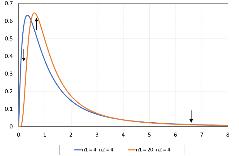
The following plot shows two probability density functions (pdfs):
the blue line is the pdf of an F random variable with parameters
![]() and
and
![]() ;
;
the orange line is the pdf of an F random variable with parameters
![]() and
and
![]() .
.
By increasing the first parameter from
![]() to
to
![]() ,
the mean of the distribution (vertical line) does not change.
,
the mean of the distribution (vertical line) does not change.
However, part of the density is shifted from the tails to the center of the distribution.
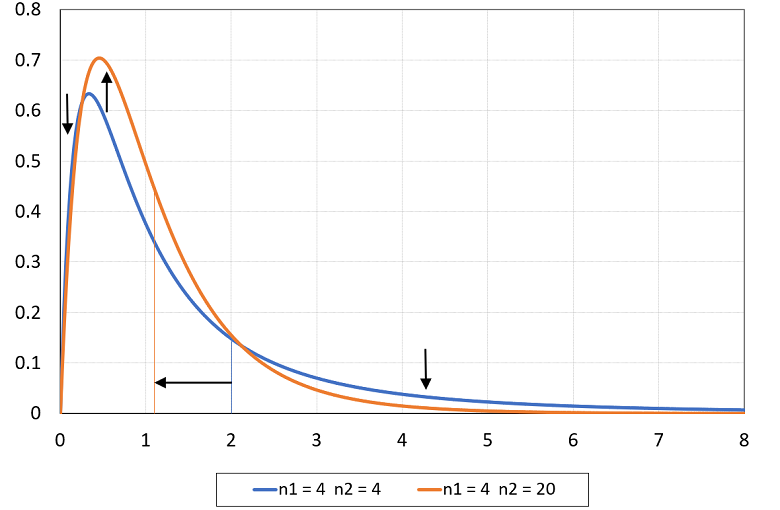
In the following plot:
the blue line is the density of an F distribution with parameters
![]() and
and
![]() ;
;
the orange line is the density of an F distribution with parameters
![]() and
and
![]() .
.
By increasing the second parameter from
![]() to
to
![]() ,
the mean of the distribution (vertical line) decreases (from
,
the mean of the distribution (vertical line) decreases (from
![]() to
to
![]() )
and some density is shifted from the tails (mostly from the right tail) to the
center of the distribution.
)
and some density is shifted from the tails (mostly from the right tail) to the
center of the distribution.
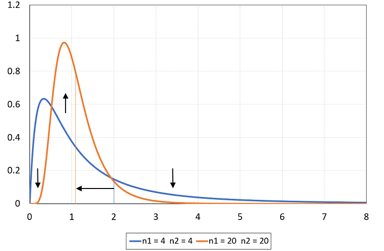
In the next plot:
the blue line is the density of an F random variable with parameters
![]() and
and
![]() ;
;
the orange line is the density of an F random variable with parameters
![]() and
and
![]() .
.
By increasing the two parameters, the mean of the distribution decreases (from
![]() to
to
![]() )
and density is shifted from the tails to the center of the distribution. As a
result, the distribution has a bell shape similar to the shape of the
normal distribution.
)
and density is shifted from the tails to the center of the distribution. As a
result, the distribution has a bell shape similar to the shape of the
normal distribution.
Below you can find some exercises with explained solutions.
Let
![]() be a Gamma random variable with parameters
be a Gamma random variable with parameters
![]() and
and
![]() .
.
Let
![]() be another Gamma random variable, independent of
be another Gamma random variable, independent of
![]() ,
with parameters
,
with parameters
![]() and
and
![]() .
.
Find the expected value of the
ratio
We can
writewhere
![]() and
and
![]() are two independent Gamma random variables, the parameters of
are two independent Gamma random variables, the parameters of
![]() are
are
![]() and
and
![]() and the parameters of
and the parameters of
![]() are
are
![]() and
and
![]() (see the lecture entitled Gamma
distribution). By using this fact, the ratio can be written
aswhere
(see the lecture entitled Gamma
distribution). By using this fact, the ratio can be written
aswhere
![]() has an F distribution with parameters
has an F distribution with parameters
![]() and
and
![]() .
Therefore,
.
Therefore,
Find the third moment of an F random variable with parameters
![]() and
and
![]() .
.
We need to use the formula for the
![]() -th
moment of an F random
variable:
-th
moment of an F random
variable:
Plugging in the parameter values, we
obtainwhere
we have used the relation between the Gamma
function and the factorial function.
Phillips, P. C. B. (1982) The true characteristic function of the F distribution, Biometrika, 69, 261-264.
Please cite as:
Taboga, Marco (2021). "F distribution", Lectures on probability theory and mathematical statistics. Kindle Direct Publishing. Online appendix. https://www.statlect.com/probability-distributions/F-distribution.
Most of the learning materials found on this website are now available in a traditional textbook format.